Haskell and functional programming

Enjoy learning haskell but not only haskell.

Haskell Introduction

In this course we use Haskell, because it is the most widespread language with good support for mathematically structured programming.

f :: Int -> Bool
f x = (x > 0)

First $x$ is the input and the RHS of the equation is the Output.

Currying

In mathematics, we treat $log_{10}(x)$ and $log_2 (x)$ and ln(x) as separate functions.

In Haskell, we have a single function logBase that, given a number n, produces a function for $log_n(x)$

log10 :: Double -> Double
log10 = logBase 10

log2 :: Double -> Double
log2 = logBase 2

ln :: Double -> Double
ln = logBase 2.71828

logBase :: Double -> Double -> Double

Function application associates to the left in Haskell, so:

logBase 2 64 ≡ (logBase 2) 64

Functions of more than one argument are usually written this way in Haskell, but it is possible to use tuples instead…

Tuples

Tuples are another way to take multiple inputs or produce multiple outputs:

toCartesian :: (Double, Double) -> (Double, Double)
toCartesian (r, theta) = (x, y)
  where x = r * cos theta
        y = r * sin theta

N.B: The order of bindings doesn’t matter. Haskell functions have no side effects, they just return a result. There’s no notion of time(no notion of sth happen before sth else).

Higher Order Functions

In addition to returning functions, functions can take other functions as arguments:

twice :: (a -> a) -> (a -> a)
twice f a = f (f a)

double :: Int -> Int
double x = x * 2

quadruple :: Int -> Int
quadruple = twice double

Haskell concrete types are written in upper case like Int, Bool, and in lower case if they stand for any type.

{-
  twice twice double 3
 == (twice twice double) 3
 == (twice (twice double)) 3
 == (twice quadruple) 3
 == quadrauple (quadruple 3)
 == 48
-}

Lists

Haskell makes extensive use of lists, constructed using square brackets. Each list element must be of the same type.

[True, False, True] :: [Bool]
[3, 2, 5+1]         :: [Int]
[sin, cos]          :: [Double -> Double]
[ (3,’a’),(4,’b’) ] :: [(Int, Char)]

Map

A useful function is map, which, given a function, applies it to each element of a list:

map not [True, False, True] = [False, True, False]
map negate [3, -2, 4]       = [-3, 2, -4]
map (\x -> x + 1) [1, 2, 3] = [2, 3, 4]

The last example here uses a lambda expression to define a one-use function without giving it a name.

What’s the type of map?

map :: (a -> b) -> [a] -> [b]

Strings

The type String in Haskell is just a list of characters:

type String = [Char]

This is a type synonym, like a typedef in C.

Thus: "hi!" == ['h', 'i', '!']

Practice

Word Frequencies

Given a number $n$ and a string $s$, generate a report (in String form) that lists the $n$ most common words in the string $s$.

We must:

• Break the input string into words.
• Convert the words to lowercase.
• Sort the words.
• Count adjacent runs of the same word.
• Sort by size of the run.
• Take the first $n$ runs in the sorted list.
• Generate a report.

import Data.Char(toLower)
import Data.List(group,sort,sortBy)

breakIntoWords :: String -> [String]
breakIntoWords = words

convertIntoLowercase :: [[Char]] -> [String]
convertIntoLowercase = map (map toLower)

sortWords :: [String] -> [String]
sortWords = sort

type Run = (Int, String)
countAdjacentRuns :: [String] -> [Run]
countAdjacentRuns = convertToRuns . groupAdjacentRuns 

-- ["hello","hello","world"] --> [["hello","hello"],["world"]]

groupAdjacentRuns :: [String] -> [[String]]
groupAdjacentRuns = group

-- head :: [a] -> a

convertToRuns :: [[String]] -> [Run]
convertToRuns = map (\ls-> (length ls, head ls))

sortByRunSize :: [Run] -> [Run]
sortByRunSize = sortBy (\(l1, w1) (l2, w2) -> compare l2 l1)

takeFirst :: Int -> [Run] -> [Run]
takeFirst = take 

generateReport :: [Run] -> String
generateReport = unlines . map (\(l,w) -> w ++ ":" ++ show l  ) 

-- (\x -> f x) == f

mostCommonWords :: Int -> (String -> String)
mostCommonWords n =
     generateReport
   . takeFirst n
   . sortByRunSize 
   . countAdjacentRuns
   . sortWords
   . convertIntoLowercase  
   . breakIntoWords

Functional Composition

We used function composition to combine our functions together. The mathematical $(f ◦ g)(x)$ is written $(f . g) x$ in Haskell.

In Haskell, operators like function composition are themselves functions. You can define your own!

-- Vector addition
(.+) :: (Int, Int) -> (Int, Int) -> (Int, Int)
(x1, y1) .+ (x2, y2) = (x1 + x2, y1 + y2)
(2,3) .+ (1,1) == (3,4)

You could even have defined function composition yourself if it didn’t already exist:

(.) :: (b -> c) -> (a -> b) -> (a -> c)
(f . g) x = f (g x)

Lists

How were all of those list functions we just used implemented?

Lists are singly-linked lists in Haskell.

The empty list is written as [] and a list node is written as x : xs.

The value x is called the head and the rest of the list xs is called the tail. Thus:

"hi!" == ['h', 'i', '!'] == 'h':('i':('!':[]))
                         == 'h' : 'i' : '!' : []

When we define recursive functions on lists, we use the last form for pattern matching:

map :: (a -> b) -> [a] -> [b]
map f []     = []
map f (x:xs) = f x : map f xs

We can evaluate programs equationally:

{-
map toUpper "hi!" ≡ map toUpper (’h’:"i!")
                  ≡ toUpper ’h’ : map toUpper "i!"
                  ≡ ’H’ : map toUpper "i!"
                  ≡ ’H’ : map toUpper (’i’:"!")
                  ≡ ’H’ : toUpper ’i’ : map toUpper "!"
                  ≡ ’H’ : ’I’ : map toUpper "!"
                  ≡ ’H’ : ’I’ : map toUpper (’!’:"")
                  ≡ ’H’ : ’I’ : ’!’ : map toUpper ""
                  ≡ ’H’ : ’I’ : ’!’ : map toUpper []
                  ≡ ’H’ : ’I’ : ’!’ : []
                  ≡ "HI!"
-}

List Functions

-- in maths: f(g(x)) == (f o g)(x)

myMap :: (a -> b) -> [a] -> [b]
myMap f []     = []
myMap f (x:xs) = (f x)  :  (myMap f xs)

-- 1 : 2 : 3 : []
-- 1 + 2 + 3 + 0
sum' :: [Int] -> Int
sum' []     = 0
sum' (x:xs) = x + sum xs


-- ["hello","world","!"] -> "helloworld!"
-- "hello":"world":"!":[]
-- "hello"++"world"++"!"++[]

concat' :: [[a]] -> [a]
concat' []        = []
concat' (xs:xss)  = xs ++ concat xss

foldr' :: (a -> b -> b) -> b -> [a] -> b
foldr' f z []     = z
foldr' f z (x:xs) = x `f` (foldr' f z xs)

sum'' = foldr' (+) 0
concat'' = foldr' (++) []

filter' :: (a -> Bool) -> [a] -> [a]
filter' p [] = []
-- filter' p (x:xs) = if p x then x : filter' p xs 
--                          else filter' p xs
filter' p (x:xs) 
   | p x       = x : filter' p xs
   | otherwise = filter' p xs

Induction

Suppose we want to prove that a property $P(n)$ holds for all natural numbers $n$. Remember that the set of natural numbers $N$ can be defined as follows:

Definition of Natural Numbers

Inductive definition of Natural numbers

1. 0 is a natural number.
2. For any natural number $n, n + 1$ is also a natural number

Therefore, to show $P(n)$ for all $n$, it suffices to show:

1. $P(0)$ (the base case), and

2. assuming $P(k)$ (the inductive hypothesis),

   $⇒ P(k + 1)$ (the inductive case).

Induction on Lists

Haskell lists can be defined similarly to natural numbers

Definition of Haskell Lists

1. [] is a list.
2. For any list xs, x:xs is also a list (for any item x).

This means, if we want to prove that a property P(ls) holds for all lists ls, it suffices to show:

1. P([]) (the base case)
2. P(x:xs) for all items x, assuming the inductive hypothesis P(xs)

Data Types

So far, we have seen type synonyms using the type keyword. For a graphics library, we might define:

type Point  = (Float, Float)
type Vector = (Float, Float)
type Line   = (Point, Point)
type Colour = (Int, Int, Int, Int) -- RGBA
movePoint :: Point -> Vector -> Point
movePoint (x,y) (dx,dy) = (x + dx, y + dy)

But these definitions allow Points and Vectors to be used interchangeably, increasing the likelihood of errors.

We can define our own compound types using the data keyword:

data Point = Point Float Float
deriving (Show, Eq)

First Point is the type name

Second Point is Constructor name

Floats are Constructor argument types

data Vector = Vector Float Float
deriving (Show, Eq)
movePoint :: Point -> Vector -> Point
movePoint (Point x y) (Vector dx dy)
= Point (x + dx) (y + dy)

Records

We could define Colour similarly:

data Colour = Colour Int Int Int Int

But this has so many parameters, it’s hard to tell which is which. Haskell lets us declare these types as records, which is identical to the declaration style on the previous slide, but also gives us projection functions and record syntax:

data Colour = Colour { redC :: Int
                      , greenC :: Int
                      , blueC :: Int
                      , opacityC :: Int
                      } deriving (Show, Eq)

Here, the code redC (Colour 255 128 0 255) gives 255.

Enumeration Types

Similar to enums in C and Java, we can define types to have one of a set of predefined values:

data LineStyle = Solid
                | Dashed
                | Dotted
                deriving (Show, Eq)
data FillStyle = SolidFill | NoFill
                  deriving (Show, Eq)

Types with more than one constructor are called sum types

Algebraic Data Types

Just as the Point constructor took two Float arguments, constructors for sum types can take parameters too, allowing us to model different kinds of shape:

data PictureObject
    = Path [Point] Colour LineStyle
    | Circle Point Float Colour LineStyle FillStyle
    | Polygon [Point] Colour LineStyle FillStyle
    | Ellipse Point Float Float Float
              Colour LineStyle FillStyle
    deriving (Show, Eq)
type Picture = [PictureObject]

Recursive and Parametric Types

Data types can also be defined with parameters, such as the well known Maybe type, defined in the standard library:

data Maybe a = Just a | Nothing

Types can also be recursive. If lists weren’t already defined in the standard library, we could define them ourselves:

data List a = Nil | Cons a (List a)

We can even define natural numbers, where 2 is encoded as Succ(Succ Zero):

data Natural = Zero | Succ Natural

Types in Design

Make illegal states unrepresentable.

​ – Yaron Minsky (of Jane Street)

Choose types that constrain your implementation as much as possible. Then failure scenarios are eliminated automatically.

Partial Functions

A partial function is a function not defined for all possible inputs.

Partial functions are to be avoided, because they cause your program to crash if undefined cases are encountered. To eliminate partiality, we must either:

• enlarge the codomain, usually with a Maybe type:

  safeHead :: [a] -> Maybe a 
  safeHead (x:xs) = Just x
  safeHead [] = Nothing

• constrain the domain to be more specific:

  safeHead' :: NonEmpty a -> a
  safeHead' (One a)    = a
  safeHead' (Cons a _) = a
  data NonEmpty a = One a | Cons a (NonEmpty a)

Type Classes

You have already seen functions such as: compare, (==), (+), (show)

that work on multiple types, and their corresponding constraints on type variables Ord, Eq, Num and Show.

These constraints are called type classes, and can be thought of as a set of types for which certain operations are implemented.

Show

The Show type class is a set of types that can be converted to strings.

class Show a where -- nothing to do with OOP
  show :: a -> String

Types are added to the type class as an instance like so:

instance Show Bool where
  show True = "True"
  show False = "False"

We can also define instances that depend on other instances:

instance Show a => Show (Maybe a) where
  show (Just x) = "Just " ++ show x
  show Nothing = "Nothing"

Fortunately for us, Haskell supports automatically deriving instances for some classes, including Show.

Read

Type classes can also overload based on the type returned.

class Read a where
  read :: String -> a

Semigroup

A semigroup is a pair of a set S and an operation • : S → S → S where the operation

• s associative.

Associativity is defined as, for all a, b, c:

(a • (b • c)) = ((a • b) • c)

Haskell has a type class for semigroups! The associativity law is enforced only by programmer discipline:

class Semigroup s where
(<>) :: s -> s -> s
-- Law: (<>) must be associative.

What instances can you think of? Lists & ++, numbers and +, numbers and *

Example:

Lets implement additive colour mixing:

instance Semigroup Colour where
Colour r1 g1 b1 a1 <> Colour r2 g2 b2 a2
     = Colour (mix r1 r2)
              (mix g1 g2)
              (mix b1 b2)
              (mix a1 a2)
where
  mix x1 x2 = min 255 (x1 + x2)

Observe that associativity is satisfied.

Moniod

A monoid is a semigroup (S, •) equipped with a special identity element z : S such that x • z = x and z • y = y for all x, y.

class (Semigroup a) => Monoid a where
  mempty :: a
For colours, the identity element is transparent black:
instance Monoid Colour where
  mempty = Colour 0 0 0 0

For each of the semigroups discussed previously(lists, num and +, num and *):

• Are they monoids? Yes
• If so, what is the identity element? [], 0, 1

Are there any semigroups that are not monoids? Maximum

Newtypes

There are multiple possible monoid instances for numeric types like Integer:

• The operation (+) is associative, with identity element 0
• The operation (*) is associative, with identity element 1

Haskell doesn’t use any of these, because there can be only one instance per type per class in the entire program (including all dependencies and libraries used).

A common technique is to define a separate type that is represented identically to the original type, but can have its own, different type class instances.

In Haskell, this is done with the newtype keyword.

A newtype declaration is much like a data declaration except that there can be only one constructor and it must take exactly one argument:

newtype Score = S Integer
instance Semigroup Score where
  S x <> S y = S (x + y)
instance Monoid Score where
  mempty = S 0

Here, Score is represented identically to Integer, and thus no performance penalty is incurred to convert between them.

In general, newtypes are a great way to prevent mistakes. Use them frequently!

Ord

Ord is a type class for inequality comparison

class Ord a where
 (<=) :: a -> a -> Bool

What laws should instances satisfy?

For all x, y, and z:

• Reflexivity: x <= x
• Transitivity: If x <= y and y <= z then x <= z
• Antisymmetry: If x <= y and y <= x then x == y.
• Totality: Either x <= y or y <= x

Relations that satisfy these four properties are called total orders(most are total orders). Without the fourth (totality), they are called partial orders(e.g. division).

Eq

Eq is a type class for equality or equivalence

class Eq a where
  (==) :: a -> a -> Bool

What laws should instances satisfy?

For all x, y, and z:

• Reflexivity: x == x.
• Transitivity: If x == y and y == z then x == z.
• Symmetry: If x == y then y == x.

Relations that satisfy these are called equivalence relations.

Some argue that the Eq class should be only for equality, requiring stricter laws like:

If x == y then f x == f y for all functions f

But this is debated.

Funtors

Types and Values

Haskell is actually comprised of two languages.

• The value-level language, consisting of expressions such as if, let, 3 etc.
• The type-level language, consisting of types Int, Bool, synonyms like String, and type constructors like Maybe, (->), [ ] etc

This type level language itself has a type system!

Kinds

Just as terms in the value level language are given types, terms in the type level language are given kinds.

The most basic kind is written as *.

• Types such as Int and Bool have kind *.
• Seeing as Maybe is parameterised by one argument, Maybe has kind * -> *: given a type (e.g. Int), it will return a type (Maybe Int).

Lists

Suppose we have a function:

toString :: Int -> String

And we also have a function to give us some numbers:

getNumbers :: Seed -> [Int]

How can I compose toString with getNumbers to get a function f of type Seed -> [String]?

we use map: f = map toString . getNumbers.

What about return a Maybe Int? we can use maybe map

maybeMap :: (a -> b) -> Maybe a -> Maybe b
maybeMap f Nothing = Nothing
maybeMap f (Just x) = Just (f x)

maybeMap f mx = case mx of
                  Nothing -> Nothing
                  Just x  -> Just (f x)

We can generalise this using functor.

Functor

All of these functions are in the interface of a single type class, called Functor.

class Functor f where
  fmap :: (a -> b) -> f a -> f b

Unlike previous type classes we’ve seen like Ord and Semigroup, Functor is over types of kind * -> *.

-- Instance for tuples
-- type level:
-- (,) :: * -> (* -> *)
-- (,) x :: * -> *
instance Functor ((,) x) where
--  fmap :: (a -> b) -> f a -> f b
--  fmap :: (a -> b) -> (,) x a -> (,) x b
--  fmap :: (a -> b) -> (x,a) -> (x, b)
  fmap f (x,a) = (x, f a)
  
-- instance for functions
-- type level:
-- (->) :: * -> (* -> *)
-- (->) x :: * -> *

instance Functor ((->) x) where
--  fmap :: (a -> b) -> f a -> f b
--  fmap :: (a -> b) -> (->) x a -> (->) x b
--  fmap :: (a -> b) -> (x -> a) -> (x -> b)
  fmap = (.)

Functor Laws

The functor type class must obey two laws:

• fmap id == id(indentity law)
• fmap f . fmap g == fmap (f . g)(composition law, haskell use this law to do optimisation)

In Haskell’s type system it’s impossible to make a total fmap function that satisfies the first law but violates the second.

This is due to parametricity.

Property Based Testing

Free Properties

Haskell already ensures certain properties automatically with its language design and type system.

• Memory is accessed where and when it is safe and permitted to be accessed (memory safety).
• Values of a certain static type will actually have that type at run time.
• Programs that are well-typed will not lead to undefined behaviour (type safety).
• All functions are pure: Programs won’t have side effects not declared in the type. (purely functional programming)

⇒ Most of our properties focus on the logic of our program.

Logical Properties

We have already seen a few examples of logical properties.

Example:

• reverse is an involution: reverse (reverse xs) == xs
• right identity for (++): xs ++ [] == xs
• transitivity of (>): (a > b) ∧ (b > c) ⇒ (a > c)

The set of properties that capture all of our requirements for our program is called the functional correctness specification of our software.

This defines what it means for software to be correct.

Proofs

Last week we saw some proof methods for Haskell programs. We could prove that our implementation meets its functional correctness specification.

Such proofs certainly offer a high degree of assurance, but:

• Proofs must make some assumptions about the environment and the semantics of the software.
• Proof complexity grows with implementation complexity, sometimes drastically.
• If software is incorrect, a proof attempt might simply become stuck: we do not always get constructive negative feedback.
• Proofs can be labour and time intensive ($$$), or require highly specialised knowledge ($$$).

Testing

Compared to proofs:

• Tests typically run the actual program, so requires fewer assumptions about the language semantics or operating environment.
• Test complexity does not grow with implementation complexity, so long as the specification is unchanged.
• Incorrect software when tested leads to immediate, debuggable counter examples.
• Testing is typically cheaper and faster than proving.
• Tests care about efficiency and computability, unlike proofs(e.g. termination is provable but not computable).

We lose some assurance, but gain some convenience ($$$).

Property Based Testing

Key idea: Generate random input values, and test properties by running them.

Example(QuickCheck Property)

import Test.QuickCheck
import Data.Char
import Data.List
--                 Testable          
--                 Arbitrary    Testable
--                               Arbitrary    Testable
prop_reverseApp :: [Int]     -> ([Int]     -> Bool)
prop_reverseApp xs ys =
   reverse (xs ++ ys) == reverse ys ++ reverse xs

divisible :: Int -> Int -> Bool
divisible x y = x `mod` y == 0
-- or select different generators with modifier newtypes.
prop_refl :: Positive Int -> Bool 
prop_refl (Positive x) = divisible x x

-- Encode pre-conditions with the (==>) operator:
prop_unwordsWords s = unwords (words s) == s
prop_wordsUnwords l = all (\w -> all (not . isSpace) w && w /= []) l 
                    ==> words (unwords l) == l

PBT vs. Unit Testing

• Properties are more compact than unit tests, and describe more cases.

  ⇒ Less testing code

• Property-based testing heavily depends on test data generation:

  • Random inputs may not be as informative as hand-crafted inputs

    ⇒ use shrinking(When a test fails, it finds the smallest test case still falls)

  • Random inputs may not cover all necessary corner cases:

    ⇒ use a coverage checker

  • Random inputs must be generated for user-defined types:

    ⇒ QuickCheck includes functions to build custom generators

• By increasing the number of random inputs, we improve code coverage in PBT.

Test Data Generation

Data which can be generated randomly is represented by the following type class:

class Arbitrary a where
  arbitrary :: Gen a -- more on this later
  shrink :: a -> [a]

Most of the types we have seen so far implement Arbitrary.

Shrinking

The shrink function is for when test cases fail. If a given input x fails, QuickCheck will try all inputs in shrink x; repeating the process until the smallest possible input is found

Testable Types

The type of the quickCheck function is:

-- more on IO later
quickCheck :: (Testable a) => a -> IO ()

The Testable type class is the class of things that can be converted into properties. This includes:

• Bool values

• QuickCheck’s built-in Property type

• Any function from an Arbitrary input to a Testable output:

  instance (Arbitrary i, Testable o)
        => Testable (i -> o) ...

Thus the type [Int] -> [Int] -> Bool (as used earlier) is Testable.

Examples

split :: [a] -> ([a],[a])
split [] = ([],[])
split [a] = ([a],[])
split (x:y:xs) = let (l,r) = split xs
                  in (x:l,y:r)


prop_splitPerm xs = let (l,r) = split (xs :: [Int])
                     in permutation xs (l ++ r)

permutation :: (Ord a) => [a] -> [a] -> Bool
permutation xs ys = sort xs == sort ys

permutation' :: (Eq a) => [a] -> [a] -> (a -> Bool)
permutation' xs ys = \x -> count x xs == count x ys
  where
    count x l = length (filter (== x) l)


merge :: (Ord a) => [a] -> [a] -> [a]
merge [] ys = ys
merge xs [] = xs
merge (x:xs) (y:ys) | x <= y    = x : merge xs (y:ys)
                    | otherwise = y : merge (x:xs) ys

prop_mergePerm xs ys = permutation (xs ++ (ys :: [Int] )) (merge xs ys)

prop_mergeSorted (Ordered xs) (Ordered ys) = sorted (merge (xs :: [Int]) ys)

sorted :: Ord a => [a] -> Bool
sorted [] = True 
sorted [x] = True
sorted (x:y:xs) = x <= y && sorted (y:xs)


mergeSort :: (Ord a) => [a] -> [a]
mergeSort [] = []
mergeSort [x] = [x]
mergeSort xs = let (l,r) = split xs
                in merge (mergeSort l) (mergeSort r)


prop_mergeSortSorts xs = sorted (mergeSort (xs :: [Int])) 

prop_mergeSortPerm xs = permutation xs (mergeSort (xs :: [Int]))

prop_mergeSortExtra xs = mergeSort (xs :: [Int]) == sort xs

prop_mergeSortUnit = mergeSort [3,2,1] == [1,2,3]


main = do
  quickCheck prop_mergeSortUnit
  quickCheck prop_mergeSortSorts
  quickCheck prop_mergeSortPerm

Redundant Properties

Some properties are technically redundant (i.e. implied by other properties in the specification), but there is some value in testing them anyway:

• They may be more efficient than full functional correctness tests, consuming less computing resources to test.
• They may be more fine-grained to give better test coverage than random inputs for full functional correctness tests.
• They provide a good sanity check to the full functional correctness properties.
• Sometimes full functional correctness is not easily computable but tests of weaker properties are.

These redundant properties include unit tests. We can (and should) combine both approaches!

Lazy Evaluation

It never evaluate anything unless it has to

sumTo :: Integer -> Integer
sumTo 0 = 0
sumTo n = sumTo (n-1) + n

This crashes when given a large number. Why? Because of the growing stack frame.

sumTo' :: Integer -> Integer -> Integer
sumTo' a 0 = a
sumTo' a n = sumTo' (a+n) (n-1)
sumTo :: Integer -> Integer
sumTo 0 = 0
sumTo n = sumTo (n-1) + n
-- sumTo' 0 5
-- sumTo' (0+5) (5-1)
-- sumTo' (0+5) 4
-- sumTo' (0+5+4) (4-1)
-- sumTo' (0+5+4) 3
-- sumTo' (0+5+4+3) (3-1)
-- sumTo' (0+5+4+3) 2 -> never evaluate the first argument
-- ..

This still crashes when given a large number. Why?

This is called a space leak, and is one of the main drawbacks of Haskell’s lazy evaluation method.

Haskell is lazily evaluated, also called call-by-need.

This means that expressions are only evaluated when they are needed to compute a result for the user.

We can force the previous program to evaluate its accumulator by using a bang pattern, or the primitive operation seq:

{-# LANGUAGE BangPatterns #-}
sumTo' :: Integer -> Integer -> Integer
sumTo' !a 0 = a
sumTo' !a n = sumTo' (a+n) (n-1)
sumTo' :: Integer -> Integer -> Integer
sumTo' a 0 = a
sumTo' a n = let a' = a + n in a' `seq` sumTo' a' (n-1)

Advantages

Lazy Evaluation has many advantages:

• It enables equational reasoning even in the presence of partial functions and non-termination
• It allows functions to be decomposed without sacrificing efficiency, for example: minimum = head . sort is, depending on sorting algorithm, possibly O(n).
• It allows for circular programming and infinite data structures, which allow us to express more things as pure functions.

Infinite Data Structures

Laziness lets us define data structures that extend infinitely. Lists are a common example, but it also applies to trees or any user-defined data type:

ones = 1 : ones

Many functions such as take, drop, head, tail, filter and map work fine on infinite lists.

naturals = 0 : map (1+) naturals
--or
naturals = map sum (inits ones)
--  fibonacci numbers
fibs = 1:1:zipWith (+) fibs (tail fibs)

Data Invariants and ADTs

Structure of a Module

A Haskell program will usually be made up of many modules, each of which exports one or more data types.

Typically a module for a data type X will also provide a set of functions, called operations, on X.

• to construct the data type: c :: · · · → X
• to query information from the data type: q :: X → · · ·
• to update the data type: u :: · · · X → X

A lot of software can be designed with this structure.

Example:

module Dictionary
  ( Word
  , Definition
  , Dict
  , emptyDict
  , insertWord
  , lookup
  ) where

import Prelude hiding (Word, lookup)
import Test.QuickCheck
import Test.QuickCheck.Modifiers
-- lookup :: [(a,b)] -> a -> Maybe b
type Word = String
type Definition = String

newtype Dict = D [DictEntry]
             deriving (Show, Eq)

emptyDict :: Dict
emptyDict = D []

insertWord :: Word -> Definition -> Dict -> Dict
insertWord w def (D defs) = D (insertEntry (Entry w def) defs)
  where
    insertEntry wd (x:xs) = case compare (word wd) (word x)
                              of GT -> x : (insertEntry wd xs)
                                 EQ -> wd : xs
                                 LT -> wd : x : xs
    insertEntry wd [] = [wd]

lookup :: Word -> Dict -> Maybe Definition
lookup w (D es) = search w es
  where
    search w [] = Nothing
    search w (e:es) = case compare w (word e) of
       LT -> Nothing
       EQ -> Just (defn e)
       GT -> search w es

sorted :: (Ord a) => [a] -> Bool
sorted []  = True
sorted [x] = True
sorted (x:y:xs) = x <= y && sorted (y:xs)

wellformed :: Dict -> Bool
wellformed (D es) = sorted es

prop_insert_wf dict w d = wellformed dict ==>
                          wellformed (insertWord w d dict)

data DictEntry
  = Entry { word :: Word
          , defn :: Definition
          } deriving (Eq, Show)

instance Ord DictEntry where
  Entry w1 d1 <= Entry w2 d2 = w1 <= w2


instance Arbitrary DictEntry where
  arbitrary = Entry <$> arbitrary <*> arbitrary

instance Arbitrary Dict where
  arbitrary = do
    Ordered ds <- arbitrary
    pure (D ds)

prop_arbitrary_wf dict = wellformed dict

Data Invariants

Data invariants are properties that pertain to a particular data type. Whenever we use operations on that data type, we want to know that our data invariants are maintained.

For a given data type X, we define a wellformedness predicate

$$
\text{wf :: X → Bool}
$$
For a given value x :: X, wf x returns true iff our data invariants hold for the value x

For each operation, if all input values of type X satisfy wf, all output values will satisfy wf.

In other words, for each constructor operation c :: · · · → X, we must show wf (c · · ·), and for each update operation u :: X → X we must show wf x =⇒ wf(u x)

Abstract Data Types

An abstract data type (ADT) is a data type where the implementation details of the type and its associated operations are hidden.

newtype Dict
type Word = String
type Definition = String
emptyDict  :: Dict
insertWord :: Word -> Definition -> Dict -> Dict
lookup     :: Word -> Dict -> Maybe Definition

If we don’t have access to the implementation of Dict, then we can only access it via the provided operations, which we know preserve our data invariants. Thus, our data invariants cannot be violated if this module is correct.

In general, abstraction is the process of eliminating detail.

The inverse of abstraction is called refinement.

Abstract data types like the dictionary above are abstract in the sense that their implementation details are hidden, and we no longer have to reason about them on the level of implementation.

Validation

Suppose we had a sendEmail function

sendEmail :: String -- email address
          -> String -- message
          -> IO () -- action (more in 2 wks)

It is possible to mix the two String arguments, and even if we get the order right, it’s possible that the given email address is not valid.

We could define a tiny ADT for validated email addresses, where the data invariant is that the contained email address is valid:

module EmailADT(Email, checkEmail, sendEmail)
    newtype Email = Email String
    checkEmail :: String -> Maybe Email
    checkEmail str | '@' `elem` str = Just (Email str)
                   | otherwise      = Nothing
-- Then, change the type of sendEmail:
    sendEmail :: Email -> String -> IO()

The only way (outside of the EmailADT module) to create a value of type Email is to use checkEmail.

checkEmail is an example of what we call a smart constructor: a constructor that enforces data invariants.

Data Refinement

Reasoning about ADTs

Consider the following, more traditional example of an ADT interface, the unbounded queue:

data Queue
emptyQueue :: Queue
enqueue :: Int -> Queue -> Queue
front   :: Queue -> Int -- partial
dequeue :: Queue -> Queue -- partial
size    :: Queue -> Int

We could try to come up with properties that relate these functions to each other without reference to their implementation, such as:

dequeue (enqueue x emptyQueue) == emptyQueue

However these do not capture functional correctness (usually).

Models for ADTs

We could imagine a simple implementation for queues, just in terms of lists:

emptyQueueL = []
enqueueL a  = (++ [a])
frontL      = head
dequeueL    = tail
sizeL       = length

But this implementation is O(n) to enqueue! Unacceptable!

However!(This is out mental model)

This is a dead simple implementation, and trivial to see that it is correct. If we make a better queue implementation, it should always give the same results as this simple one. Therefore: This implementation serves as a functional correctness specification for our Queue type!

Refinement Relations

The typical approach to connect our model queue to our Queue type is to define a relation, called a refinement relation, that relates a Queue to a list and tells us if the two structures represent the same queue conceptually:

rel :: Queue -> [Int] -> Bool
prop_empty_r = rel emptyQueue emptyQueueL
prop_size_r fq lq = rel fq lq ==> size fq == sizeL lq
prop_enq_ref fq lq x = rel fq lq ==> rel (enqueue x fq) (enqueueL x lq)

Abstraction Functions

These refinement relations are very difficult to use with QuickCheck because the rel fq lq preconditions are very hard to satisfy with randomly generated inputs. For this example, it’s a lot easier if we define an abstraction function that computes the corresponding abstract list from the concrete Queue.

toAbstract :: Queue → [Int]

Conceptually, our refinement relation is then just:

\fq lq → absfun fq == lq

However, we can re-express our properties in a much more QC-friendly format

import Test.QuickCheck


emptyQueueL = []
enqueueL a  = (++ [a])
frontL      = head
dequeueL    = tail
sizeL       = length


toAbstract :: Queue -> [Int]
toAbstract (Q f sf r sr) = f ++ reverse r

prop_empty_ref = toAbstract emptyQueue == emptyQueueL

prop_enqueue_ref fq x = toAbstract (enqueue x fq)
                     == enqueueL x (toAbstract fq)

prop_size_ref fq = size fq == sizeL (toAbstract fq)

prop_front_ref fq = size fq > 0 ==> front fq == frontL (toAbstract fq)
prop_deq_ref fq = size fq > 0 ==>  toAbstract (dequeue fq)
                                == dequeueL (toAbstract fq)

prop_wf_empty = wellformed emptyQueue
prop_wf_enq x q = wellformed q ==> wellformed (enqueue x q)
prop_wf_deq x q = wellformed q && size q > 0 ==> wellformed (dequeue q)

data Queue = Q [Int] -- front of the queue
               Int   -- size of the front
               [Int] -- rear of the queue
               Int   -- size of the rear
             deriving (Show, Eq)

wellformed :: Queue -> Bool
wellformed (Q f sf r sr) = length f == sf && length r == sr
                        && sf >= sr

instance Arbitrary Queue where
  arbitrary = do
    NonNegative sf' <- arbitrary
    NonNegative sr <- arbitrary
    let sf = sf' + sr
    f <- vectorOf sf arbitrary
    r <- vectorOf sr arbitrary
    pure (Q f sf r sr)


inv3 :: Queue -> Queue
inv3 (Q f sf r sr)
   | sf < sr   = Q (f ++ reverse r) (sf + sr) [] 0
   | otherwise = Q f sf r sr

emptyQueue :: Queue
emptyQueue = Q [] 0 [] 0

enqueue :: Int -> Queue -> Queue
enqueue x (Q f sf r sr) = inv3 (Q f sf (x:r) (sr+1))

front :: Queue -> Int   -- partial
front (Q (x:f) sf r sr) = x

dequeue :: Queue -> Queue -- partial
dequeue (Q (x:f) sf r sr) = inv3 (Q f (sf -1) r sr)

size    :: Queue -> Int
size (Q f sf r sr) = sf + sr

Data Refinement

These kinds of properties establish what is known as a data refinement from the abstract, slow, list model to the fast, concrete Queue implementation.

Refinement and Specifications

In general, all functional correctness specifications can be expressed as:

• all data invariants are maintained, and
• the implementation is a refinement of an abstract correctness model.

There is a limit to the amount of abstraction we can do before they become useless for testing (but not necessarily for proving).

Effects

Effects are observable phenomena from the execution of a program.

Internal vs. External Effects

External Observability

An external effect is an effect that is observable outside the function. Internal effects are not observable from outside.

Example

Console, file and network I/O; termination and non-termination; non-local control flow; etc.

Are memory effects external or internal?

Depends on the scope of the memory being accessed. Global variable accesses are external.

Purity

A function with no external effects is called a pure function.

A pure function is the mathematical notion of a function. That is, a function of type a -> b is fully specified by a mapping from all elements of the domain type a to the codomain type b.

Consequences:

• Two invocations with the same arguments result in the same value.
• No observable trace is left beyond the result of the function.
• No implicit notion of time or order of execution.

Haskell Functions

Haskell functions are technically not pure.

• They can loop infinitely.

• They can throw exceptions (partial functions)

• They can force evaluation of unevaluated expressions.

Caveat

Purity only applies to a particular level of abstraction. Even ignoring the above, assembly instructions produced by GHC aren’t really pure.

Despite the impurity of Haskell functions, we can often reason as though they are pure. Hence we call Haskell a purely functional language.

The Danger of Implicit Side Effects

• They introduce (often subtle) requirements on the evaluation order.
• They are not visible from the type signature of the function.
• They introduce non-local dependencies which is bad for software design, increasing coupling.
• They interfere badly with strong typing, for example mutable arrays in Java, or reference types in ML.

We can’t, in general, reason equationally about effectful programs!

Can we program with pure functions?

Typically, a computation involving some state of type s and returning a result of type a can be expressed as a function:

s -> (s, a)

Rather than change the state, we return a new copy of the state.

All that copying might seem expensive, but by using tree data structures, we can usually reduce the cost to an O(log n) overhead.

State

State Passing

data Tree a = Branch a (Tree a) (Tree a) | Leaf
-- Given a tree, label each node with an ascending number in infix order:
label :: Tree () -> Tree Int
lable t = snd (go t 1)
	where 
		go :: Tree() -> Int -> (Int, Tree Int)
		go Leaf c = (c, Leaf)
		go (Branch () l r) c = let
        (c', l') = go l c
        v = c'
        (c'', r') = go r (c'+1)
      in (c'', Branch v l' r')
-- it works but not pretty

Let’s use a data type to simplify this!

State

newtype State s a = A procedure that, manipulating some state of type s, returns a
-- State Operations
get :: State s s
put :: s -> State s ()
pure :: a -> State s a
evalState :: State s a -> s -> a
-- Sequential Composition
-- Do one state action after another with do blocks:
do put 42 desugars put 42 >> put True
pure True
(>>) :: State s a -> State s b -> State s b
-- Bind
-- The 2nd step can depend on the first with bind:
do x <- get desugars get >>= \x -> pure (x + 1)
pure (x+1)
(>>=) :: State s a -> (a -> State s b) -> State s b

Example

{-
modify :: (s -> s) -> State s ()
modify f = do
  s <- get
  put (f s)
-}

label' :: Tree () -> Tree Int
label' t = evalState (go t) 1 
  where
    go :: Tree () -> State Int (Tree Int)
    go Leaf = pure Leaf
    go (Branch () l r) = do
       l' <- go l
       v  <- get
       put (v + 1)
       r' <- go r
       pure (Branch v l' r')

newtype State' s a = State (s -> (s, a))

get' :: State' s s
get' = (State $ \s -> (s, s))  

put' :: s -> State' s ()
put' s = State $ \_ -> (s,())

pure' :: a -> State' s a
pure' a = State $ \s -> (s, a)

evalState' :: State' s a -> s -> a
evalState (State f) s = snd (f s) 

(>>=!) :: State' s a -> (a -> State' s b) -> State' s b
(State c) >>=! f = State $ \s -> let (s', a) = c s
                                    (State c') = f a
                                 in c' s'

(>>!) :: State' s a -> State' s b -> State' s b
(>>!) a b = a >>=! \_ -> b

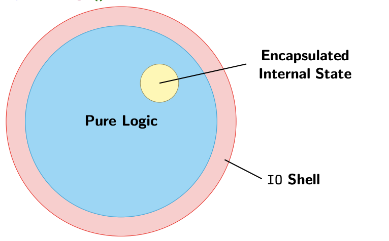
IO

A procedure that performs some side effects, returning a result of type a is written as IO a.

IO a is an abstract type. But we can think of it as a function:

RealWorld -> (RealWorld, a)

(that’s how it’s implemented in GHC)

(>>=) :: IO a -> (a -> IO b) -> IO b
pure  :: a -> IO a

getChar :: IO Char
readLine :: IO String
putStrLn :: String -> IO () -- return a procedure

Infectious IO

We can convert pure values to impure procedures with pure:

pure :: a -> IO a

But we can’t convert impure procedures to pure values

The only function that gets an a from an IO a is >>=:

(>>=) :: IO a -> (a -> IO b) -> IO b

But it returns an IO procedure as well.

If a function makes use of IO effects directly or indirectly, it will have IO in its type!

Haskell Design Strategy

We ultimately “run” IO procedures by calling them from main:

main :: IO ()

Example

-- Given an input number n, print a triangle of * characters of base width n.
printTriangle :: Int -> IO ()
printTriangle 0 = pure ()
printTriangle n = do
  putStrLn (replicate n '*')
  printTriangle (n - 1)

main = printTriangle 9

{-
Design a game that reads in a n × n maze from a file. The player starts at position
(0, 0) and must reach position (n − 1, n − 1) to win. The game accepts keyboard input
to move the player around the maze.
-}
import Data.List 
import System.IO

mazeSize :: Int 
mazeSize = 10

data Tile = Wall | Floor deriving (Show, Eq)


type Point = (Int, Int)


lookupMap :: [Tile] -> Point -> Tile
lookupMap ts (x,y) = ts !! (y * mazeSize + x)

addX :: Int -> Point -> Point
addX dx (x,y) = (x + dx, y)

addY :: Int -> Point -> Point
addY dy (x,y) = (x, y + dy)

data Game = G { player :: Point
              , map    :: [Tile]
              }

invariant :: Game -> Bool 
invariant (G (x,y) ts) = x >= 0 && x < mazeSize
                      && y >= 0 && y < mazeSize
                      && lookupMap ts (x,y) /= Wall

moveLeft :: Game -> Game 
moveLeft (G p m) 
  = let g' = G (addX (-1) p) m
     in if invariant g' then g' else G p m

moveRight :: Game -> Game
moveRight (G p m) 
  = let g' = G (addX 1 p) m
     in if invariant g' then g' else G p m

moveUp :: Game -> Game
moveUp (G p m)
  = let g' = G (addY (-1) p) m
     in if invariant g' then g' else G p m

moveDown :: Game -> Game
moveDown (G p m) 
  = let g' = G (addY 1 p) m
     in if invariant g' then g' else G p m

won :: Game -> Bool 
won (G p m) = p == (mazeSize-1,mazeSize-1)

main :: IO () 
main = do 
    str <- readFile "input.txt"
    let initial = G (0,0) (stringToMap str)
    gameLoop initial
  where 
    gameLoop :: Game -> IO () 
    gameLoop state 
        | won state = putStrLn "You win!"
        | otherwise = do 
            display state
            c <- getChar' 
            case c of 
                'w' -> gameLoop (moveUp state)
                'a' -> gameLoop (moveLeft state)
                's' -> gameLoop (moveDown state)
                'd' -> gameLoop (moveRight state)
                'q' -> pure ()
                _   -> gameLoop state 

stringToMap :: String -> [Tile]
stringToMap [] = []
stringToMap ('#':xs) = Wall : stringToMap xs 
stringToMap (' ':xs) = Floor : stringToMap xs 
stringToMap (c:xs)   = stringToMap xs

display :: Game -> IO () 
display (G (px,py) m) = printer (0,0) m 
  where 
    printer (x,y) (t:ts) = do 
        if (x,y) == (px,py) then putChar '@'
        else if t == Wall then putChar '#'
        else putChar ' '

        if (x == mazeSize - 1) then do
            putChar '\n'
            printer (0,y+1) ts 
        else printer (x+1,y) ts
    printer (x,y) [] = putChar '\n'

getChar' :: IO Char 
getChar' = do 
    b <- hGetBuffering stdin 
    e <- hGetEcho stdin
    hSetBuffering stdin NoBuffering
    hSetEcho stdin False
    x <- getChar 
    hSetBuffering stdin b
    hSetEcho stdin e
    pure x

Benefits of an IO Type

• Absence of effects makes type system more informative:
  • A type signatures captures entire interface of the function
  • All dependencies are explicit in the form of data dependencies.
  • All dependencies are typed
• It is easier to reason about pure code and it is easier to test
  • Testing is local, doesn’t require complex set-up and tear-down.
  • Reasoning is local, doesn’t require state invariants
  • Type checking leads to strong guarantees.

Mutable Variables

We can have honest-to-goodness mutability in Haskell, if we really need it, using IORef.

data IORef a
newIORef :: a -> IO (IORef a)
readIORef :: IORef a -> IO a
writeIORef :: IORef a -> a -> IO ()

Example

import Data.IORef 
import Test.QuickCheck.Monadic 
import Test.QuickCheck

averageListIO :: [Int] -> IO Int
averageListIO ls = do 
    sum <- newIORef 0
    count <- newIORef 0
    let loop :: [Int] -> IO ()
        loop [] = pure ()
        loop (x:xs) = do 
            s <- readIORef sum 
            writeIORef sum (s + x) 
            c <- readIORef count 
            writeIORef count (c + 1) 
            loop xs 
    loop ls 
    s <- readIORef sum 
    c <- readIORef count 
    pure (s `div` c)    

prop_average :: [Int] -> Property
prop_average ls = monadicIO $ do 
    pre (length ls > 0)
    avg <- run (averageListIO ls)
    assert (avg == (sum ls `div` length ls))

Mutable Variables, Locally

Something like averaging a list of numbers doesn’t require external effects, even if we use mutation internally.

data STRef s a
newSTRef :: a -> ST (STRef s a)
readSTRef :: STRef s a -> ST s a
writeSTRef :: STRef s a -> a -> ST s ()
runST :: (forall s. ST s a) -> a

The extra s parameter is called a state thread, that ensures that mutable variables don’t leak outside of the ST computation.

The ST type is not assessable in this course, but it is useful sometimes in Haskell programming.

QuickChecking Effects

QuickCheck lets us test IO (and ST) using this special property monad interface:

monadicIO :: PropertyM IO () -> Property
pre       :: Bool -> PropertyM IO ()
assert    :: Bool -> PropertyM IO ()
run       :: IO a -> PropertyM IO a

Do notation and similar can be used for PropertyM IO procedures just as with State s and IO procedures.

Example

-- GNU Factor
import Test.QuickCheck 
import Test.QuickCheck.Modifiers
import Test.QuickCheck.Monadic 
import System.Process

-- readProcess :: FilePath -> [String] -> String -> IO String

test_gnuFactor :: Positive Integer -> Property
test_gnuFactor (Positive n) = monadicIO $ do
    str <- run (readProcess "gfactor" [show n] "")
    let factors = map read (tail (words str))
    assert (product factors == n)

Functor

Recall the type class defined over type constructors called Functor.

We’ve seen instances for lists, Maybe, tuples and functions.

Other instances include:

• IO (how?)
• States (how?)
• Gen

ioMap :: (a -> b) -> IO a -> IO b
ioMap f act = do 
	a <- act
	pure (f a)
	
stateMap :: (a -> b) -> State s a -> State s b
stateMap f act = do 
	a <- act
	pure (f a)

-- more general
monadMap :: Monad m => (a -> b) -> m a -> m b
monadMap f act = do 
	a <- act
	pure (f a)

QuickCheck Generators

{-
class Arbitrary a where
	arbitray :: Gen a
	shrink   :: a -> [a]
-- Gen a ~=~ random generator of values type a.
-}

sortedLists :: (Arbitrary a, Ord a) => Gen [a]
sortedLists = fmap sort arbitrary :: Gen a
-- listOf :: Gen a -> Gen [a]

Applicative Functors

Binary Functions

Suppose we want to look up a student’s zID and program code using these functions:

lookupID :: Name -> Maybe ZID
lookupProgram :: Name -> Maybe Program
--  we had a function:
makeRecord :: ZID -> Program -> StudentRecord

How can we combine these functions to get a function of type Name -> Maybe StudentRecord?

lookupRecord :: Name -> Maybe StudentRecord
lookupRecord n = let zid     = lookupID n
                     program = lookupProgram n
                 in ?

Binary Map?

We could imagine a binary version of the maybeMap function:

maybeMap2 :: (a -> b -> c)
          -> Maybe a -> Maybe b -> Maybe c

But then, we might need a trinary version.

maybeMap3 :: (a -> b -> c -> d)
          -> Maybe a -> Maybe b -> Maybe c -> Maybe d

Or even a 4-ary version, 5-ary, 6-ary. . . this would quickly become impractical!

Using Functor?

Using fmap gets us part of the way there:

lookupRecord' :: Name -> Maybe (Program -> StudentRecord)
lookupRecord' n = let zid     = lookupID n
                      program = lookupProgram n
                  in fmap makeRecord zid
                  -- what about program?

But, now we have a function inside a Maybe.

Applicative

This is encapsulated by a subclass of Functor called Applicative.

class Functor f => Applicative f where
  pure :: a -> f a
  (<*>) :: f (a -> b) -> f a -> f b

Maybe is an instance, so we can use this for lookupRecord:

lookupRecord :: Name -> Maybe StudentRecord
lookupRecord n = let zid     = lookupID n
                     program = lookupProgram n
                 in fmap makeRecord zid <*> program
                 -- or pure makeRecord <*> zid <*> program

Using Applicative

In general, we can take a regular function application:
$$
\text{f a b c d}
$$
And apply that function to Maybe (or other Applicative) arguments using this pattern (where <*> is left-associative):

$$
\text{pure f <*> ma <*> mb <*> mc <*> }
$$

Relationship to Functor

All law-abiding instances of Applicative are also instances of Functor, by defining:

fmap f x = pure f <*> x

Sometimes this is written as an infix operator, <$>, which allows us to write:

pure f <*> ma <*> mb <*> mc <*> md
-- as:
f <$> ma <*> mb <*> mc <*> md

Applicative laws

-- Identity
pure id <*> v = v
-- Homomorphism
pure f <*> pure x = pure (f x)
-- Interchange
u <*> pure y = pure ($ y) <*> u
-- Composition
pure (.) <*> u <*> v <*> w = u <*> (v <*> w)

Example

type Name = String
type ZID = Int
data Program = COMP | SENG | BINF | CENG deriving (Show, Eq)
type StudentRecord = (Name, ZID, Program)

lookupID :: Name -> Maybe ZID
lookupID "Liam" = Just 3253158
lookupID "Unlucky" = Just 4444444
lookupID "Prosperous" = Just 8888888
lookupID _ = Nothing

lookupProgram :: Name -> Maybe Program
lookupProgram "Liam" = Just COMP
lookupProgram "Unlucky" = Just SENG
lookupProgram "Prosperous" = Just CENG
lookupProgram _ = Nothing

makeRecord :: ZID -> Program -> Name -> StudentRecord
makeRecord zid pr name = (name,zid,pr)



liam :: Maybe StudentRecord
liam = let mzid = lookupID "Liam"
           mprg = lookupProgram "Liam"
        in pure makeRecord <*> mzid <*> mprg <*> pure "Liam"

--     pure :: a -> Maybe a
--     fmap :: (a -> b) -> Maybe a -> Maybe b

Functor Laws for Applicative

These are proofs not Haskell code:

fmap f x = pure f <*> x

-- The two functor laws are:
1. fmap id x == x
2. fmap f (fmap g x) == fmap (f.g) x


-- Proof:

1) pure id <*> x == x -- true by Identity law

2) pure f <*> (pure g <*> x)
     == pure (.) <*> pure f <*> pure g <*> x --Composition
     == pure ((.) f) <*> pure g <*> x        --Homomorphism
     == pure (f.g) <*> x                     --Homomorphism

Applicative Lists

There are two ways to implement Applicative for lists:

(<*>) :: [a -> b] -> [a] -> [b]

• Apply each of the given functions to each of the given arguments, concatenating all the results
• Apply each function in the list of functions to the corresponding value in the list of arguments

The second one is put behind a newtype (ZipList) in the Haskell standard library.

pureZ :: a -> [a]
pureZ a = a:pureZ a

applyListsZ :: [a -> b] -> [a] -> [b]
applyListsZ (f:fs) (x:xs) = f x : applyListsZ fs xs
applyListsZ [] _ = []
applyListsZ _ [] = []

pureC :: a -> [a]
pureC a = [a] 

applyListsC :: [a -> b] -> [a] -> [b]
applyListsC (f:fs) args = map f args ++ applyListsC fs args
applyListsC [] args = []

Other instances

QuickCheck generators: Gen

data Concrete = C [Char] [Char]
  deriving (Show, Eq)
instance Arbitrary Concrete where
  arbitrary = C <$> arbitrary <*> arbitrary

Functions: ((->) x

The Applicative instance for functions lets us pass the same argument into multiple functions without repeating ourselves.

instance Applicative ((->) x) where
  pure :: a -> x -> a
  pure a x = a

  (<*>) :: (x -> (a -> b)) -> (x -> a) -> (x -> b)
  (<*>) xab xa x = xab x (xa x)

-- f (g x) (h x) (i x)
--
-- Can be written as: 
-- (pure f <*> g <*> h <*> i) x

Tuples: ((,) x)

We can’t implement pure without an extra constraint!

The tuple instance for Applicative lets us combine secondary outputs from functions into one secondary output without manually combining them.

instance Functor ((,) x) where
  fmap :: (a -> b) -> (x,a) -> (x,b)
  fmap f (x,a) = (x,f a)

-- monoid has an identity element
instance Monoid x => Applicative ((,) x) where
  pure :: a -> (x,a)
  pure a = (mempty ,a)

  (<*>) :: (x,a -> b) -> (x, a) -> (x, b)
  (<*>) (x, f) (x',a) = (x <> x', f a)

It requires Monoid here to combine the values, and to provide a default value for pure.

f :: A -> (Log, B)
g :: X -> (Log, Y)
a :: A
x :: X
combine :: B -> Y -> Z

-- combine the logs silently
test :: (Log, Z)
test = combine <$> f a <*> g x
-- instead of 
--  let (l1, b) = f a
--      (l2, y) = g x
--   in (l1 <> l2, combine b y)

IO and State s

instance Applicative IO where
	pure :: a -> IO a
	pure a = pure a 
	
	(<*>) :: IO (a -> b) -> IO a -> IO b
	pf <*> pa = do
		f <- pf
		a <- pa
		pure (f a)

Monads

Monads are types m where we can sequentially compose functions of the form a -> m b

class Applicative m => Monad m where
  (>>=) :: m a -> (a -> m b) -> m b

Sometimes in old documentation the function return is included here, but it is just an alias for pure. It has nothing to do with return as in C/Java/Python etc.

Example

-- Maybe Monad
(>>=) :: Maybe a -> (a -> Maybe b) -> Maybe b
(>>=) Nothing f = Nothing
(>>=) (Just a) f = f a

-- List Monad
(>>=) :: [a] -> (a -> [b]) -> [b]
(>>=) as f = concatMap f as

-- function
(>>=) :: (x -> a) -> (a -> x ->b) -> b
(>>=) xa axb x = axb (xa x) x

-- function monad example(reader monad)
f :: A -> Config -> B
f :: X -> Config -> Y
f :: B -> Config -> C

combine :: (A, X) -> Config -> (Y, C)
combine (a, x) = do
	b <- f a
	y <- g x
	c <- h b
	pure(y, c)

Monad Law

We can define a composition operator with (>>=):

(<=<) :: (b -> m c) -> (a -> m b) -> (a -> m c) 
(f <=< g) x = g x >>= f

Monad Laws

f <=< (g <=< x) == (f <=< g) <=< x -- associativity
pure <=< f      == f               -- left identity
f <=< pure      == f               -- right identity

These are similar to the monoid laws, generalised for multiple types inside the monad. This sort of structure is called a category in mathematics.

Relationship to Applicative

All Monad instances give rise to an Applicative instance, because we can define <*> in terms of >>=.

mf <*> mx = mf >>= \f -> mx >>= \x -> pure (f x)

This implementation is already provided for Monads as the ap function in Control.Monad

Do notation

Working directly with the monad functions can be unpleasant. As we’ve seen, Haskell has some notation to increase niceness:

do x <- y  
									becomes y >>= \x -> do z
   z

do x
                  becomes x >>= \_ -> do y
   y

Examples

{-
 (Dice Rolls)
 Roll two 6-sided dice, if the difference is < 2, reroll the second   die. Final score is the
 difference of the two die. What score is most common?
-}
roll :: [Int]
roll = [1, 2, 3, 4, 5, 6]

diceGame = do
	d1 <- roll
	d2 <- roll
	if (abs (d1 - d2) < 2) then do
		d2' <- roll
		pure (abs (d1 - d2'))
	else 
	  pure (abs (d1 - d2))
	  
{-
 Partial Functions
 We have a list of student names in a database of type [(ZID, Name)]. Given a list of
 zID’s, return a Maybe [Name], where Nothing indicates that a zID could not be found
-}
db :: [(ZID, Name)]
db = [(3253158, "Liam"),
      (8888888, "Rich"),
      (4444444, "Mort")]

studentNames :: [ZID] -> Maybe [Name]
studentNames [] = pure []
studentNames (z:zs) = do 
     n  <- lookup z db
     ns <- studentNames zs
     pure (n:ns)

-- briefer but less clear with applicative notation:
-- studentNames (z:zs) = (:) <$> lookup z db <*> studentNames zs

{-
 Arbitrary Instances
 Define a Tree type and a generator for search trees:
 searchTrees :: Int -> Int -> Generator Tree
-}
data Tree a = Leaf 
            | Branch a (Tree a) (Tree a) 
            deriving (Show, Eq)

instance Arbitrary (Tree Int) where
  arbitrary = do
      mn <- (arbitrary :: Gen Int)
      Positive delta <- arbitrary
      let mx = mn + delta
      searchTree mn mx
    where
      searchTree :: Int -> Int -> Gen (Tree Int)
      searchTree mn mx 
         | mn >= mx = pure Leaf
         | otherwise = do
            v <- choose (mn,mx)
            l <- searchTree mn v
            r <- searchTree (v+1) mx
            pure (Branch v l r)

-- The Either Monad
studentNames :: [ZID] -> Either ZID [Name]
studentNames [] = pure []
studentNames (z:zs) = do 
     n  <- case lookup z db of
             Just v -> Right v
             Nothing -> Left z
     ns <- studentNames zs
     pure (n:ns)

Static Assurance with Types

Static Assureance

Methods of Assurance

Static means of assurance analyse a program without running it.

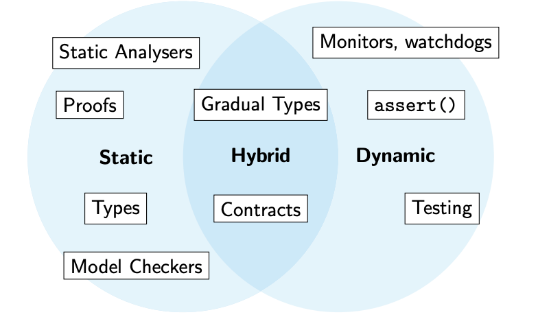
Static vs. Dynamic

Static checks can be exhaustive.

Exhaustivity

An exhaustive check is a check that is able to analyse all possible executions of a program.

• However, some properties cannot be checked statically in general (halting problem), or are intractable to feasibly check statically (state space explosion).
• Dynamic checks cannot be exhaustive, but can be used to check some properties where static methods are unsuitable.

Compiler Integration

Most static and all dynamic methods of assurance are not integrated into the compilation process.

• You can compile and run your program even if it fails tests
• You can change your program to diverge from your model checker model.
• Your proofs can diverge from your implementation.

Types

Because types are integrated into the compiler, they cannot diverge from the source code. This means that type signatures are a kind of machine-checked documentation for your code.

Types are the most widely used kind of formal verification in programming today.

• They are checked automatically by the compiler.
• They can be extended to encompass properties and proof systems with very high expressivity (covered next week).
• They are an exhaustive analysis

Phantom Types

A type parameter is phantom if it does not appear in the right hand side of the type definition.

newtype Size x = S Int

Lets examine each one of the following use cases:

• We can use this parameter to track what data invariants have been established about a value.
• We can use this parameter to track information about the representation (e.g. units of measure).
• We can use this parameter to enforce an ordering of operations performed on these values (type state).

Validation

Suppose we have

data UG -- empty type
data PG
data StudentID x = SID Int

We can define a smart constructor that specialises the type parameter:

sid :: Int -> Either (StudentID UG)
                     (StudentID PG)

Define functions:

enrolInCOMP3141 :: StudentID UG -> IO ()
lookupTranscript :: StudentID x -> IO String

Units of Measure

data Kilometres
data Miles
data Value x = U Int
sydneyToMelbourne = (U 877 :: Value Kilometres)
losAngelesToSanFran = (U 383 :: Value Miles)
-- Note the arguments to area must have the same unit
data Square a
area :: Value m -> Value m -> Value (Square m)
area (U x) (U y) = U (x * y)

Type State

{-
  A Socket can either be ready to recieve data, or busy. If the socket is busy, the user
  must first use the wait operation, which blocks until the socket is ready. If the socket
  is ready, the user can use the send operation to send string data, which will make the
  socket busy again.
-}
data Busy
data Ready
newtype Socket s = Socket ...
wait :: Socket Busy -> IO (Socket Ready)
send :: Socket Ready -> String -> IO (Socket Busy)
-- assumption: use the socket in a linear way(only use once)

Linearity and Type State

The previous code assumed that we didn’t re-use old Sockets:

send2 :: Socket Ready -> String -> String
       -> IO (Socket Busy)
send2 s x y = do s' <- send s x
                 s'' <- wait s'
                 s''' <- send s'' y
                 pure s'''
-- But we can just re-use old values to send without waiting:
send2' s x y = do _ <- send s x
                 s' <- send s y
                 pure s'

Linear type systems can solve this, but not in Haskell (yet)

Datatype Promotion

data UG
data PG
data StudentID x = SID Int

Defining empty data types for our tags is untyped. We can have StudentID UG, but also StudentID String.

The DataKinds language extension lets us use data types as kinds:

{-# LANGUAGE DataKinds, KindSignatures #-}
data Stream = UG | PG
data StudentID (x :: Stream) = SID Int

postgrad :: [Int]
postgrad = [3253158]

makeStudentID :: Int -> Either (StudentID UG) (StudentID PG)
makeStudentID i | i `elem` postgrad = Right (SID i) 
                | otherwise         = Left  (SID i)

enrollInCOMP3141 :: StudentID UG -> IO ()
enrollInCOMP3141 (SID x) 
  = putStrLn (show x ++ " enrolled in COMP3141!")

GADTs

Untyped Evaluator

data Expr t = BConst Bool
            | IConst Int
            | Times (Expr Int) (Expr Int)
            | Less (Expr Int) (Expr Int)
            | And (Expr Bool) (Expr Bool)
            | If (Expr Bool) (Expr t) (Expr t)
            deriving (Show, Eq)
data Value = BVal Bool | IVal Int
             deriving (Show, Eq)

eval :: Expr -> Value
eval (BConst b) = BVal b
eval (IConst i) = IVal i
eval (Times e1 e2) = case (eval e1, eval e2) of 
                       (IVal i1, IVal i2) -> IVal (i1 * i2)
eval (Less e1 e2)  = case (eval e1, eval e2) of
                       (IVal i1, IVal i2) -> BVal (i1 < i2) 
eval (And e1 e2)  = case (eval e1, eval e2) of
                       (BVal b1, BVal b2) -> BVal (b1 && b2) 
eval (If ec et ee) = 
  case eval ec of 
    BVal True  -> eval et
    BVal False -> eval ee
-- partial function
eval :: Expr -> Maybe Value
eval (BConst b) = pure (BVal b)
eval (IConst i) = pure (IVal i)
eval (Times e1 e2) = do
     v1 <- eval e1
     v2 <- eval e2
     case (v1,v2) of
       (IVal v1', IVal v2') -> pure (IVal (v1' * v2'))
       _ -> Nothing
eval (Less e1 e2) = do
     v1 <- eval e1
     v2 <- eval e2
     case (v1,v2) of
       (IVal v1', IVal v2') -> pure (BVal (v1' < v2'))
       _ -> Nothing
eval (And e1 e2) = do
     v1 <- eval e1
     v2 <- eval e2
     case (v1,v2) of
       (BVal v1', BVal v2') -> pure (BVal (v1' && v2'))
       _ -> Nothing
eval (If ec et ee) = do
     v1 <- eval ec
     case v1 of
       (BVal True) -> eval et
       (BVal False) -> eval ee

GADTs

Generalised Algebraic Datatypes (GADTs) is an extension to Haskell that, among other things, allows data types to be specified by writing the types of their constructors.

{-# LANGUAGE GADTs, KindSignatures #-}
-- Unary natural numbers, e.g. 3 is S (S (S Z))
data Nat = Z | S Nat
-- is the same as
data Nat :: * where
Z :: Nat
S :: Nat -> Nat

When combined with the type indexing trick of phantom types, this becomes very powerful!

Typed Evaluator

There is now only one set of precisely-typed constructors.

{-# LANGUAGE GADTs, KindSignatures #-}
data Expr :: * -> * where
  BConst :: Bool -> Expr Bool
  IConst :: Int -> Expr Int
  Times  :: Expr Int -> Expr Int -> Expr Int
  Less   :: Expr Int -> Expr Int -> Expr Bool
  And    :: Expr Bool -> Expr Bool -> Expr Bool
  If     :: Expr Bool -> Expr a -> Expr a -> Expr a

eval :: Expr t -> t
eval (IConst i)    = i
eval (BConst b)    = b
eval (Times e1 e2) = eval e1 * eval e2
eval (Less e1 e2)  = eval e1 < eval e2
eval (And e1 e2)   = eval e1 && eval e2
eval (If ec et ee) = if eval ec then eval et else eval ee

Lists

We could define our own list type using GADT syntax as follows:

data List (a :: *) :: * where
Nil :: List a
Cons :: a -> List a -> List a
-- head (hd) and tail (tl) functions are partial 
hd (Cons x xs) = x
tl (Cons x xs) = xs

We will constrain the domain of these functions by tracking the length of the list on the type level.

Vectors

{-# LANGUAGE GADTs, KindSignatures #-}
{-# LANGUAGE DataKinds, StandaloneDeriving, TypeFamilies #-}

data Nat = Z | S Nat

plus :: Nat -> Nat -> Nat 
plus Z n = n
plus (S m) n = S (plus m n)

type family Plus (m :: Nat) (n :: Nat) :: Nat where
  Plus Z n = n
  Plus (S m) n = S (Plus m n)

data Vec (a :: *) :: Nat -> * where
  Nil :: Vec a Z
  Cons :: a -> Vec a n -> Vec a (S n)

deriving instance Show a => Show (Vec a n)

appendV :: Vec a m -> Vec a n -> Vec a (Plus m n)
appendV Nil ys         = ys
appendV (Cons x xs) ys = Cons x (appendV xs ys)

-- 0: Z
-- 1: S Z
-- 2: S (S Z)

hd :: Vec a (S n) -> a
hd (Cons x xs) = x

mapVec :: (a -> b) -> Vec a n -> Vec b n
mapVec f Nil = Nil
mapVec f (Cons x xs) = Cons (f x) (mapVec f xs)

Tradeoffs

The benefits of this extra static checking are obvious, however:

• It can be difficult to convince the Haskell type checker that your code is correct, even when it is.
• Type-level encodings can make types more verbose and programs harder to understand.
• Sometimes excessively detailed types can make type-checking very slow, hindering productivity

Pragmatism

We should use type-based encodings only when the assurance advantages outweigh the clarity disadvantages.

The typical use case for these richly-typed structures is to eliminate partial functions from our code base.

If we never use partial list functions, length-indexed vectors are not particularly useful

Theory of Types

Logic

We can specify a logical system as a _deductive system_ by providing a set of rules and axioms that describe how to prove various connectives.

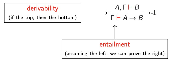
Natural Deduction

A way we can specify logic

Each connective typically has introduction and elimination rules. For example, to prove an implication A → B holds, we must show that B holds assuming A. This introduction rule is written as:

More rules

Implication also has an elimination rule, that is also called modus ponens:
$$\frac{\ulcorner \vdash A\rightarrow B \space\space\space\space\space\space\space\space\ulcorner \vdash A}{\ulcorner \vdash B}\rightarrow-E$$
Conjunction (and) has an introduction rule that follows our intuition:
$$
\frac{\ulcorner \vdash A\space\space\space\space\space\space\space\space\space \ulcorner \vdash B}{\ulcorner \vdash A\land B}\land-I_1
$$
It has two elimination rules:
$$
\frac{\ulcorner \vdash A\land B}{\ulcorner \vdash A}\land-E_1\space\space\space\space\space\space\space\space\space\space\frac{\ulcorner \vdash A\land B}{\ulcorner \vdash B}\land-E_2
$$
Disjunction (or) has two introduction rules:
$$
\frac{\ulcorner \vdash A}{\ulcorner \vdash A\lor B}\land-I_1\space\space\space\space\space\space\space\space\space\space\frac{\ulcorner \vdash A}{\ulcorner \vdash A\lor B}\land-I_2
$$
Disjunction elimination is a little unusual:
$$
\frac{\ulcorner \vdash A\lor B\space\space\space\space\space\space\space A,\ulcorner \vdash P \space\space\space\space\space\space\space B,\ulcorner \vdash P}{\ulcorner \vdash P}\lor-E
$$
The true literal, written T, has only an introduction:
$$
\frac{}{\ulcorner \vdash \top}
$$
And false, written ⊥, has just elimination (ex falso quodlibet):
$$
\frac{\ulcorner \vdash \bot}{\ulcorner \vdash P}
$$
Typically we just define：
$$
\neg A \equiv(A\rightarrow\bot)
$$

Constructive Logic

The logic we have expressed so far does not admit the law of the excluded middle:
$$
P\lor\neg P
$$
Or the equivalent double negation elimination:
$$
(\neg\neg P)\rightarrow P
$$
This is because it is a constructive logic that does not allow us to do proof by contradiction.

Typed Lambda Calculus

Boiling Haskell Down

The theoretical properties we will describe also apply to Haskell, but we need a smaller language for demonstration purposes.

• No user-defined types, just a small set of built-in types.
• No polymorphism (type variables)
• Just lambdas (λx.e) to define functions or bind variables.

This language is a very minimal functional language, called the simply typed lambda calculus, originally due to Alonzo Church.

Our small set of built-in types are intended to be enough to express most of the data types we would otherwise define.

We are going to use logical inference rules to specify how expressions are given types (typing rules).

Function Types

We create values of a function type A → B using lambda expressions:
$$
\frac{x :: A, \ulcorner\vdash e::B}{\ulcorner\vdash\lambda x.e::A\rightarrow B}
$$
The typing rule for function application is as follows:
$$
\frac{\ulcorner\vdash e_1:: A\rightarrow B\space\space\space\space\space\space\space\space \ulcorner\vdash e_2::A}{\ulcorner\vdash e_1 e_2:: B}
$$

Composite Data Types

In addition to functions, most programming languages feature ways to compose types together to produce new types, such as: Classes, Tuples, Structs, Unions, Records…

Product Types

For simply typed lambda calculus, we will accomplish this with tuples, also called product types. (A, B)

We won’t have type declarations, named fields or anything like that. More than two values can be combined by nesting products, for example a three dimensional vector:
$$
\text{(Int, (Int, Int))}
$$

Constructors and Eliminators

We can construct a product type the same as Haskell tuples:
$$
\frac{\ulcorner\vdash e_1:: A\space\space\space\space\space\space\space\space \ulcorner\vdash e_2::B}{\ulcorner\vdash(e_1, e_2):: (A, B)}
$$
The only way to extract each component of the product is to use the fst and snd eliminators:
$$
\frac{\ulcorner\vdash e:: (A,B)}{\ulcorner\vdash \text{fst }e::A}\space\space\space\space\space\space\space\space \frac{\ulcorner\vdash e:: (A,B)}{\ulcorner\vdash \text{snd }e::B}
$$

Unit Types

Currently, we have no way to express a type with just one value. This may seem useless at first, but it becomes useful in combination with other types. We’ll introduce the unit type from Haskell, written (), which has exactly one inhabitant, also written ():
$$
\frac{}{\ulcorner\vdash ():: ()}
$$

Disjunctive Composition

We can’t, with the types we have, express a type with exactly three values.

data TrafficLight = Red | Amber | Green

In general we want to express data that can be one of multiple alternatives, that contain different bits of data.

type Length = Int
type Angle = Int
data Shape = Rect Length Length
           | Circle Length | Point
           | Triangle Angle Length Length

Sum Types

We’ll build in the Haskell Either type to express the possibility that data may be one of two forms.
$$
\text{Either } A \space B
$$
These types are also called sum types.

Our TrafficLight type can be expressed (grotesquely) as a sum of units:
$$
\text{TrafficLight } \simeq \text{Either () (Either () ())}
$$

Constructors and Eliminators for Sums

To make a value of type Either A B, we invoke one of the two constructors:
$$
\frac{\ulcorner\vdash e:: A}{\ulcorner\vdash \text{Left }e::\text{Either }A\space B} \space\space\space\space \space\space\space\space \frac{\ulcorner\vdash e:: B}{\ulcorner\vdash \text{Right }e::\text{Either }A\space B}
$$
We can branch based on which alternative is used using pattern matching:
$$
\frac{\ulcorner\vdash e::\text{Either }A\space B\space\space\space \space \space\space\space\space x::A,\ulcorner\vdash e_1::P\space \space\space\space\space\space\space\space y::B,\ulcorner\vdash e_2::P}{\ulcorner\vdash (\textbf{case }e\textbf{ of}\text{ Left x}\rightarrow e_1; \text{ Right y}\rightarrow e_2)::P}
$$
Example

Our traffic light type has three values as required:
$$
\begin{align*}
\text{TrafficLight } &\simeq \text{Either () (Either () ())}\\
\text{Red } &\simeq \text{Left ()}\\
\text{Amber } &\simeq \text{Right (Left ())}\\
\text{Green } &\simeq \text{Right (Right (Left ()}\\
\end{align*}
$$

The Empty Type

We add another type, called Void, that has no inhabitants. Because it is empty, there is no way to construct it.

We do have a way to eliminate it, however:
$$
\frac{\ulcorner\vdash e::\text{Void}}{\ulcorner\vdash \text{absurd }e::P}
$$
If I have a variable of the empty type in scope, we must be looking at an expression that will never be evaluated. Therefore, we can assign any type we like to this expression, because it will never be executed.

Gathering Rules

$$
\frac{\ulcorner\vdash e::\text{Void}}{\ulcorner\vdash \text{absurd }e::P}\space\space\space\space\space\space\frac{}{\ulcorner\vdash ():: ()}\\
\frac{\ulcorner\vdash e:: A}{\ulcorner\vdash \text{Left }e::\text{Either }A\space B} \space\space\space\space \space\space\space\space \frac{\ulcorner\vdash e:: B}{\ulcorner\vdash \text{Right }e::\text{Either }A\space B}\\
\frac{\ulcorner\vdash e::\text{Either }A\space B\space\space\space \space \space\space\space\space x::A,\ulcorner\vdash e_1::P\space \space\space\space\space\space\space\space y::B,\ulcorner\vdash e_2::P}{\ulcorner\vdash (\textbf{case }e\textbf{ of}\text{ Left x}\rightarrow e_1; \text{ Right y}\rightarrow e_2)::P}\\
\frac{\ulcorner\vdash e_1:: A\space\space\space\space\space\space \ulcorner\vdash e_2::B}{\ulcorner\vdash(e_1, e_2):: (A, B)}\space\space\space\space\space\space\frac{\ulcorner\vdash e:: (A,B)}{\ulcorner\vdash \text{fst }e::A}\space\space\space\space\space\space\frac{\ulcorner\vdash e:: (A,B)}{\ulcorner\vdash \text{snd }e::B}\\
\frac{\ulcorner\vdash e_1:: A\rightarrow B\space\space\space\space\space\space\ulcorner\vdash e_2::A}{\ulcorner\vdash e_1 e_2::B}\space\space\space\space\space\space\space\frac{x :: A, \ulcorner\vdash e::B}{\ulcorner\vdash\lambda x.e::A\rightarrow B}
$$

Removing Terms. . .

$$
\frac{\ulcorner\vdash\text{Void}}{\ulcorner\vdash P}\space\space\space\space\space\space\frac{}{\ulcorner\vdash ()}\\
\frac{\ulcorner\vdash A}{\ulcorner\vdash\text{Either }A\space B} \space\space\space\space \space\space\space\space \frac{\ulcorner\vdash B}{\ulcorner\vdash\text{Either }A\space B}\\
\frac{\ulcorner\vdash \text{Either }A\space B\space\space\space \space \space\space\space\space A,\ulcorner\vdash P\space \space\space\space\space\space\space\space B,\ulcorner\vdash P}{\ulcorner\vdash P}\\
\frac{\ulcorner\vdash A\space\space\space\space\space\space \ulcorner\vdash B}{\ulcorner\vdash(A, B)}\space\space\space\space\space\space\frac{\ulcorner\vdash (A,B)}{\ulcorner\vdash A}\space\space\space\space\space\space \frac{\ulcorner\vdash (A,B)}{\ulcorner\vdash B}\\
\frac{\ulcorner\vdash A\rightarrow B\space\space\space\space\space\space\ulcorner\vdash A}{\ulcorner\vdash B}\space\space\space\space\space\space\space\frac{ A, \ulcorner\vdash B}{\ulcorner\vdash A\rightarrow B}
$$

This looks exactly like constructive logic! If we can construct a program of a certain type, we have also created a proof of a program

The Curry-Howard Correspondence

This correspondence goes by many names, but is usually attributed to Haskell Curry and William Howard.

It is a very deep result:

Programming	Logic
Types	Propositions
Programs	Proofs
Evaluation	Proof Simplification

It turns out, no matter what logic you want to define, there is always a corresponding λ-calculus, and vice versa.

λ-calculus	Logic
Typed λ-Calculus	Constructive Logic
Continuations	Classical Logic
Monads	Modal Logic
Linear Types, Session Types	Linear Logic
Region Types	Separation Logic

Translating

We can translate logical connectives to types and back:

Types	logical connectives
Tuples	Conjuction($\land$)
Either	Disjunction (∨)
Functions	Implication
()	True
Void	False

We can also translate our equational reasoning on programs into proof simplification on proofs!

Proof Simplification

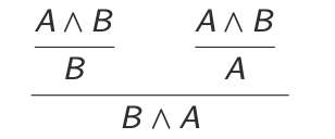
Assuming A $∧$ B, we want to prove B $∧$ A. We have this unpleasant proof:

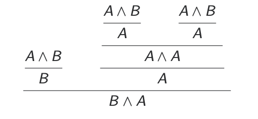
Translating to types, we get: Assuming x :: (A, B), we want to construct (B, A).

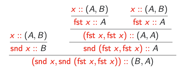
We know that
$$
\text{(snd x, snd (fst x, fst x)) = (snd x, fst x)}
$$
Assuming x :: (A, B), we want to construct (B, A).

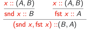
Back to logic:

Applications

As mentioned before, in dependently typed languages such as Agda and Idris, the distinction between value-level and type-level languages is removed, allowing us to refer to our program in types (i.e. propositions) and then construct programs of those types (i.e. proofs).

Generally, dependent types allow us to use rich types not just for programming, but also for verification via the Curry-Howard correspondence.

Caveats

All functions we define have to be total and terminating. Otherwise we get an inconsistent logic that lets us prove false things.

Most common calculi correspond to constructive logic, not classical ones, so principles like the law of excluded middle or double negation elimination do not hold.

Algebraic Type Isomorphism

Semiring Structure

These types we have defined form an algebraic structure called a commutative semiring

Laws for Either and Void:

• Associativity: Either (Either A B) C $\simeq$ Either A (Either B C)
• Identity: Either Void A $\simeq$ A
• Commutativity: Either A B $\simeq$ Either B A

Laws for tuples and 1:

• Associativity: ((A, B), C) $\simeq$ (A,(B, C))
• Identity: ((), A) $\simeq$ A
• Commutativity: (A, B) $\simeq$ (B, A)

Combining the two:

• Distributivity: (A, Either B C) $\simeq$ Either (A, B) (A, C)
• Absorption: (Void, A) $\simeq$ Void

What does $\simeq$ mean here? It’s more than logical equivalence. Distinguish more things.

Isomorphism

Two types A and B are isomorphic, written A $\simeq$ B, if there exists a bijection between them. This means that for each value in A we can find a unique value in B and vice versa.

Example:

data Switch = On Name Int
            | Off Name

Can be simplified to the isomorphic (Name, Maybe Int).

Generic Programming

Representing data types generically as sums and products is the foundation for generic programming libraries such as GHC generics. This allows us to define algorithms that work on arbitrary data structures.

Polymorphism and Parametricty

Type Quantifiers

Consider the type of fst:

fst :: (a,b) -> a

This can be written more verbosely as:

fst :: forall a b. (a,b) -> a

Or, in a more mathematical notation:
$$
\text{fst}::\forall a\space b(a, b)\rightarrow a
$$
This kind of quantification over type variables is called parametric polymorphism or just polymorphism for short.

(It’s also called generics in some languages, but this terminology is bad)

Curry-Howard

The type quantifier ∀ corresponds to a universal quantifier ∀, but it is not the same as the ∀ from first-order logic. What’s the difference?

First-order logic quantifiers range over a set of individuals or values, for example the natural numbers:
$$
\forall x. x+1 >x
$$
These quantifiers range over propositions (types) themselves. It is analogous to second-order logic, not first-order:
$$
\forall A.\forall B\space A\land B \rightarrow B\land A\\
\forall A.\forall B\space (A, B) \rightarrow (B, A)
$$
The first-order quantifier has a type-theoretic analogue too (type indices), but this is not nearly as common as polymorphism.

Generality

A type A is more general than a type B, often written A $\sqsubseteq$ B, if type variables in A can be instantiated to give the type B.

If we need a function of type Int → Int, a polymorphic function of type ∀a. a → a will do just fine, we can just instantiate the type variable to Int. But the reverse is not true. This gives rise to an ordering.

Example
$$
\text{Int}\rightarrow\text{Int} \sqsupseteq \forall z. z\rightarrow z\sqsupseteq \forall x\space y. x\rightarrow y\sqsupseteq\forall a. a
$$

Constraining Implementations

How many possible total, terminating implementations are there of a function of the following type? Many
$$
\text{Int}\rightarrow\text{Int}
$$
How about this type? 1
$$
\forall a. a\rightarrow a
$$

Polymorphic type signatures constrain implementations.

Parametricity

The principle of parametricity states that the result of polymorphic functions cannot depend on values of an abstracted type.

More formally, suppose I have a polymorphic function g that is polymorphic on type a. If run any arbitrary function f :: a → a on all the a values in the input of g, that will give the same results as running g first, then f on all the a values of the output.

Example:
$$
foo :: ∀a. [a] → [a]
$$
We know that every element of the output occurs in the input. The parametricity theorem we get is, for all f :
$$
\text{foo }\circ(\text{map f}) = (\text{map f})\circ \text{foo}
$$

$$
head :: ∀a. [a] → a\\
\text{ f (head l) = head (map f l)}
$$

$$
(++) :: ∀a. [a] → [a] → [a]\\
\text{map f (a ++ b) = map f a ++ map f b}
$$

$$
concat :: ∀a. [[a]] → [a]\\
\text{map f (concat ls) = concat (map (map f ) ls)}
$$

Higher Order Functions

$$
filter :: ∀a. (a → Bool) → [a] → [a]\\
\text{filter p (map f ls) = map f (filter (p ◦ f ) ls)}
$$

Parametricity Theorems

Follow a similar structure. In fact it can be mechanically derived, using the relational parametricity framework invented by John C. Reynolds, and popularised by Wadler in the famous paper, “Theorems for Free!”1 .

Upshot: We can ask lambdabot on the Haskell IRC channel for these theorems.