Foundation of Concurrency
Gain more insight about concurrency.
Semantics
Notes
Notes made by Liam. To use as a guide for revision.
Bridging the Gap
We have seen several semantic models for concurrent systems in this course. Initially, when we introduced Linear Temporal Logic, we viewed concurrent processes as sets of behaviours, where behaviours were infinite sequences of states.
This model is very nice for specifying the semantics of LTL, which we did in Week 1.
Later on, though, we used different semantic models, such as Transition Diagrams and Ben-Ari’s pseudocode. We introduced the Calculus of Communicating Systems (CCS), a type of process algebra, to construct Labelled Transition Systems, analogous to our transition diagrams. This was intended to give us a formal language that is semantically connected to our diagrammatic notation.
There is a missing link, however, between these two semantic notions: The world of CCS and labelled transition systems on one hand, and the world of behaviours and LTL properties on the other.
We examined the two CCS processes $a ⋅ (b + c)$ and $a ⋅ b + a ⋅ c$ and concluded that LTL would not be able to distinguish these two processes, even though they are not considered equal (bisimilar) in CCS.
If we were to try to add the equation $a⋅(P + Q) = a ⋅ P + a ⋅ Q$ into CCS, then we would identify those two processes above, but we would also identify $a ⋅ b + a$ with $a ⋅ b$, and clearly one of these satisfies $◊b$ and the other doesn’t!
This is because the semantic equivalence we get by adding that equation is called partial trace equivalence. As mentioned in lectures, partial trace equivalence is like looking at all the possible sequences of actions (traces) in the process, including those sequences that do not take available transitions. So, the traces of $a⋅b+a$ are $ϵ$ (the empty trace), $a$, and $ab$ – exactly the same as the partial traces of $a⋅b$.
Because partial trace equivalence includes these incomplete traces, using it is basically giving up on the vital progress assumption. Progress is the assumption that a process will take an action if one is available.
To get the set of behaviours we expect for our LTL semantics, we need some way to choose which traces we want to keep and which ones we don’t. This is the definition of what counts as a completed trace. There are many different completeness criteria. Progress is the weakest, and the most common. Other completeness criteria include weak and strong fairness, which we have seen already, and justness which I will describe below.
Progress
A simple way to view progress as a completeness criteria is that it says a path is complete iff it is infinite or if it ends in a state with no outgoing transitions. This rules out all paths which end in states where they could take an outgoing transition but don’t.
Weak Fairness
Weak and strong fairness are defined in terms of tasks. A task is a set of transitions.
Weak fairness as a property of paths can be expressed by the LTL formulas
$$
◻(◻(enabled(t))⇒◊(taken(t)))
$$
for each task tt. Here enabled(t)enabled(t) is an atomic proposition that is true if a transition in tt is enabled. Likewise taken(t)taken(t) holds if tt is taken in that state.
Given a process $P=a⋅P+b$, weak fairness would state that eventually $b$ must occur, as we would not be able to loop infinitely around $a$, never taking the (forever enabled) $b$ transition.
Viewed as a completeness criterion, weak fairness rules out all traces which do not obey the property above. Note that it implies progress, because any trace that will eventually take a forever enabled transition will surely not be able to sit in a state without taking an available transition.
Strong Fairness
Strong fairness is similar to weak fairness, except that the property has one extra operator:
$$
◻(◻◊(enabled(t))⇒◊(taken(t))))
$$
This is saying that our task tt does not have to be forever enabled, just enabled infinitely often. This means a process can go away and come back. For example, the process $P=a⋅a⋅P+b$ would not eventually do $b$ under weak fairness, as after one $a$ the $b$ transition is no longer enabled. However because the infinite aa path has $b$ available infinitely often, strong fairness would require that $b$ is eventually taken.
Viewed as a completeness criterion, this rules out all properties that don’t obey the property above. It can be proven in LTL that strong fairness implies weak fairness.
Justness
Justness is a slightly harder concept to formalise. It is weaker than both strong and weak fairness, but stronger than progress.
Essentially, it is a criterion that says that individual components should be able to make progress on their own. For example, imagine a system that consists of three components, one which always does aa, another which always does bb, and another which synchronises with aa:
$A=a⋅A$
$B=b⋅B$
$C=\bar a⋅A$
System$=A|B|C$
Now, a valid trace of this system would be simply $bbbbb⋯$ forever. This would satisfy progress, as a transition is always being taken. However, the actions $a$ and $\bar a$ that could occur, and the communication $τ$ transition that could between $A$ and $C$ are never taken in this trace. Justness says that each component of the system will always make progress if their resources are available. In other words, $B$ doing unrelated $b$ moves should never prevent $A$ and $C$ from communicating.
Viewed as a completeness criterion, this is stronger than progress, as it is essentially the same as progress except applied locally, rather than globally. It is weaker than weak fairness, as justness would not require that $A=a⋅A+b$ eventually does a $b$, as all transitions are from the same component ($A$).
Kripke Structures
These traces that we have examined are still sequences of actions, not states. Behaviours, however, are sequences of states.
Normally, to convert our labelled transition systems into something we can reason about in LTL, we first translate them into an automata called a Kripke Structure. A Kripke structure is a 4-tuple $(S,I,↦,L)$ which contains a set of states $S$, an initial state $I$, a transition relation $↦$ which, unlike a labelled transition system, does not have any action labels on the transitions, and a labelling function $L$ which associates to every state $S$ a (set of) atomic propositions – these are the atomic propositions we use in our LTL formulae. A Kripke structure for an OS process behaviour was actually shown in the lecture on temporal logic in Week 1, I just never told you it was a Kripke structure.
Kripke Structures deal with states, not transition actions. This means, to translate from a labelled transition system to a Kripke structure, we need a way to move labels from transitions to states.
The simplest translation is due to de Nicola and Vaandrager, where each transition $s_i\xrightarrow a s_j$ in the LTS is split into two in the Kripke Structure: $s_i→X$ and $X→s_j$, where $X$ is a new state that is labelled with $a$.
Because this converts existing LTS locations into blank, unlabelled states in the Kripke structure, this introduces problems with the next state operator in LTL. For this reason (and others) we usually consider LTL without the next state operator in this field.
Normally with LTL, we require that Kripke structures have no deadlock states, that is, states with no outgoing transitions. The usual solution here is to add a self loop to all terminal states.
We can extract our normal notion of a behaviour by using the progress completeness criterion. Because of the restriction above, the progress criterion is equivalent to examining only the infinite runs of the automata.
Putting it all together
Now we can:
- Translate Pseudocode to CCS or transition diagrams
- Translate transition systems to Kripke structures
- Extract behaviours from Kripke structures using various completeness criteria
- Specify LTL properties about those behaviours
Now we have connected all the semantic models used in the course.
Pseudocode
Calculus of Communicating Systems(CCS)
The Calculus of Communicating Systems:
- Is a process algebra, a simple formal language to describe concurrent systems.
- Is given semantics in terms of labelled transition systems.
- Was developed by Turing-award winner Robin Milner in the 1980s
- Has an abstract view of synchronization that applies well to message passing.
Processes
Processes in CCS are defined by equations:
The equation:
$$
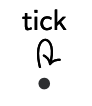
\textbf{CLOCK} = \text{tick}
$$
defines a process CLOCK that simply executes the action_ “tick” and then terminates. This process corresponds to the first location in this **_labelled transition system** (LTS):
$$
\bullet\xrightarrow{\text{tick}}\bullet
$$
An LTS is like a transition diagram, save that our transitions are just abstract actions and we have no initial or final location.
Action Prefixing
If a is an action and $P$ is a process, then $x.P$ is a process that executes $x$ before $P$. This brackets to the right, so:
$$
x.y.z.P = x.(y.(z.P))
$$
Example
$$
\textbf{CLOCK}_2 = \text{tick.tock}
$$
defines a process called CLOCK$_2$ that executes the action “tick” then the action “tock” and then terminates
$$
\bullet\xrightarrow{\text{tick}}\bullet\xrightarrow{\text{tock}}\bullet
$$
The process:
$$
\textbf{CLOCK}_3 = \text{tock.tick}
$$
has the same actions as CLOCK$_2$ but arranges them in another order.
Stopping
More precisely, we should write:
$$
\textbf{CLOCK}_2 = \text{tick.tock.}\textbf{STOP}
$$
where STOP is the trivial process with no transitions.
Loops
Up to now, all processes make a finite number of transitions and then terminate. Processes that can make a infinite number of transitions can be pictured by allowing loops:
 CLOCK$_4 =$ tick.CLOCK$_4$
 CLOCK$5_ =$ tick.tick,CLOCK$_5$
We accomplish loops in CCS using recursion.
Equality of Processes
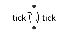
These two processes(CLOCK$_4$ and CLOCK$_5$) are physically different:
But they both have the same behaviour — an infinite sequence of “tick” transitions.
(Informal definition)
We consider two process to be equal if an external observer cannot distinguish them by their actions. We will refine this definition later.
Choice
If $P$ and $Q$ are processes then $P + Q$ is a process which can either behave as the process $P$ or the process $Q$.
Choice Equalities
$$
\begin{align}
&P + (Q + R) &= \space&(P + Q) + R &(\text{associativity})\\
&P + Q &= \space&Q + P &(\text{commutativity})\\
&P + STOP &= \space&P &(\text{neutral element})\\
&P + P &= \space&P &(\text{idempotence})
\end{align}
$$
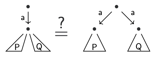
What about the equation:
$$
a.(P + Q)=^?(a.P) + (a.Q)
$$
Branching Time
Exmaple:
$\textbf{VM}_1 = \text{in}50¢.(\text{outCoke + outPepsi})$
$ \textbf{VM}_2 = (\text{in}50¢.\text{outCoke}) + (\text{in}50¢.\text{outPepsi})$
Reactive Systems
VM$_1$ allows the customer to choose which drink to vend after inserting 50¢. In VM$_2$ however, the machine makes the choice when the customer inserts a coin. They different in this reactive view, but they have the same behaviours!
Equivalences
The equation
$$
a.(P + Q) = (a.P) + (a.Q)
$$
is usually not admitted for this reason.
If we do admit it, then our notion of equality is very coarse (it is called partial trace equivalence). This is enough if we want to prove safety properties, but progress is not guaranteed.
Our notion of equality without this equation is called (strong) bisimulation equivalence or (strong) bisimilarity.
Parallel Composition
If $P$ and $Q$ are processes then $P | Q$ is the parallel composition of their processes — i.e. the non-deterministic interleaving of their actions
$$
\textbf{ACLOCK}=\text{tick.beep | tock}
$$
Synchronization
In CCS, every action a has an opposing coaction $\bar a$ (and $\bar{\bar a}$ = a):
It is a convention to think of an action as an output event and a coaction as an input event. If a system can execute both an action and its coaction, it may execute them both simultaneously by taking an internal transition marked by the special action $τ$ .
Expansion Theorem
Let $P$ and $Q$ be processes. By expanding recursive definitions and using our existing equations for choice we can express $P$ and $Q$ as n-ary choices of action prefixes:
$$
P =\sum_{i∈I}\alpha_i. P_i \text{ and } Q =\sum_{j∈J}β_j. Q_j
$$
Then, the parallel composition can be expressed as follows:
$$
P | Q =\sum_{i∈I}αi.(P_i| Q) +\sum_{j∈J}β_j.(P | Q_j) + \sum
_{i∈I, j∈J, α_i=\barβ_j}τ.(P_i| Q_j)
$$
From this, many useful equations are derivable:
$$
\begin{align}
&P|Q &= \space&Q|P\\
&P|(Q|R) &=\space &(P|Q)|R\\
&P|\text{STOP} &=\space &P\\
\end{align}
$$
Restriction
If $P$ is a process and a is an action (not $τ$ ), then $P \ a$ is the same as the process $P$ except that the actions a and a may not be executed. We have
$(a.P)$ \ $ b = a.(P $\ $ b) \text{ if } a \not\in {b, \bar b}$
Example:
$$
\begin{align}
&\textbf{CLOCK}_4 &= \space&\text{tick}\textbf{.CLOCK}_4\\
&\textbf{MAN} &=\space &\bar {\text{tick}}\text{.eat.}\textbf{MAN} \\
&\textbf{EXAMPLE} &=\space &(\textbf{MAN|CLOCK}_4)\text{\ tick}\\
\end{align}
$$
Semantics
Up until now, our semantics were given informally in terms of pictures. Now we will formalise our semantic intuitions.
Our set of locations in our labelled transition system will be the set of all CCS processes. Locations can now be labelled with what process they are:
We will now define what transitions exist in our LTS by means of a set of inference rules. This technique is called operational semantics.
Inference Rules
In logic we often write:
$$
\frac{A_1, A_2, … A_n}{C}
$$
To indicate that C can be proved by proving all assumptions A1 through An. For example, the classical logical rule of modus ponens is written as follows:
$$
\frac{A\Rightarrow B\qquad A}{B}\text{Modus Ponens}
$$
Operational Semantics
$$
\frac{}{a.P\xrightarrow{a} P}\text{ACT}\qquad
\frac{P\xrightarrow{a} P’}{P+Q\xrightarrow{a} P’}\text{CHOICE}_1\qquad
\frac{Q\xrightarrow{a} Q’}{P+Q\xrightarrow{a} Q’}\text{CHOICE}_2
$$
$$
\frac{P\xrightarrow{a} P’}{P|Q\xrightarrow{a} P’|Q}\text{PAR}_1\qquad
\frac{Q\xrightarrow{a} Q’}{P|Q\xrightarrow{a} P|Q’}\text{PAR}_2\qquad
\frac{P\xrightarrow{a} P’\quad Q\xrightarrow{a} Q’}{P|Q\xrightarrow{τ} P’|Q’}\text{SYNC}
$$
$$
\frac{P\xrightarrow{a} P’\quad a\not\in{b,\bar b}}{P\text{ \ }b\xrightarrow{a} P’\text{ \ }b}\text{RESTRICT}
$$
Bisimulation Equivalence
Two processes (or locations) P and Q are bisimilar iff they can do the same actions and those actions themselves lead to bisimilar processes. All of our previous equalities can be proven by induction on the semantics here.
Proof Trees
The advantages of this rule presentation is that they can be “stacked” to give a neat tree like derivation of proofs.

Value Passing
We introduce synchronous channels into CCS by allowing actions and coactions to take parameters.
$$
\begin{align}
&\text{Actions:}&a(3)\qquad &c(15) &x(True)…\
&\text{Coactions:}&\bar a(x)\qquad &\bar c(y) &\bar c(z)…
\end{align}
$$
The parameter of an action is the value to be sent, and the parameter of a coaction is the variable in which the received value is stored.
Example
A one-cell sized buffer is implemented as:
$$
\textbf{BUFF}=\bar{\text{in}}(x).\text{out}(x).\textbf{BUFF}
$$
Larger buffers can be made by stitching multiple BUFF processes together! This is how we model asynchronous communication in CCS.
Merge and Guards
Guard:
If $P$ is a value-passing CCS process and $ϕ$ is a formula about the variables in scope, then $[ϕ]P$ is a process that executes just like $P$ if $ϕ$ is holds for the current state and like STOP otherwise
We can define an if statement like so:
$$
\textbf{if } ϕ \textbf{ then } P \textbf{ else } Q≡ ([ϕ].P) + ([¬ϕ].Q)
$$
Assignment
If $P$ is a process and $x$ is a variable in the state, and $e$ is an expression, then $[\![x := e]\!]$ $P$ is is the same as $P$ except that it first updates the variable $x$ to have the value $e$ before making a transition.
Some presentations of value passing CCS also include assignment to update variables in the state.
With this, our value-passing CCS is now just as expressive as Ben-Ari’s pseudocode. Moreover, the connection between CCS and transition diagrams is formalised, enabling us to reason symbolically about processes rather than semantically.
Process Algebra
This is an example of a process algebra. There are many such algebras and they have been very influential on the design of concurrent programming languages.
Kripke Structures(KS)
Linear Temporal Logic(LTL)
Logic
A logic is a formal language designed to express logical reasoning. Like any formal languages, logics have a syntax and semantics(meaning of the value).
Example: Proposition Logic Syntax
A set of atomic propositions $P = {a, b, c, …}$
An inductively defined set of formulae:
- Each $p \in P$ is a formula
- If $P$ and $Q$ are formulae, then $P \land Q$ is a formula
- If $P$ is a formula, then $\neg P$ is a formula
(Other connectives(like or) are just sugar for these, so we omit them)
Sematics
Semantics are a mathematical representation of the meaning of a piece of syntax. There are many ways of giving a logic semantics, but we will use models.
Example (Propositional Logic Semantics)
A model for propositional logic is a valuation $V ⊆ P$, a set of “true” atomic propositions. We can extend a valuation over an entire formula, giving us a satisfaction relation:
$$
\begin{align}
V ⊨ p &⇔ p \in V\\
V ⊨ \varphi \land \psi &⇔ V ⊨ \varphi\text{ and }V ⊨ \psi\\
V ⊨ \neg \varphi &⇔ V |\ne \varphi
\end{align}
$$
We read $V ⊨ φ$ as $V$ “satisfies” $φ$.
LTL
Linear temporal logic (LTL) is a logic designed to describe linear time properties.
Linear temporal logic syntax
We have normal propositional operators:
- $p ∈ P$ is an LTL formula.
- If $ϕ$, $ψ$ are LTL formulae, then $ϕ ∧ ψ$ is an LTL formula.
- If $ϕ$ is an LTL formula, $¬ϕ$ is an LTL formula.
We also have modal or temporal operators:
If $ϕ$ is an LTL formula, then $\circ ϕ$ is an LTL formula.
The circle is read as ‘next’
If $ϕ$, $ψ$ are LTL formulae, then $ϕ U ψ$ is an LTL formula.
The U is read as until.
LTL Semantics
let $\sigma = \sigma_0\sigma_1\sigma_2\sigma_3\sigma_4\sigma_5…$ be a behavior. Then define the notation:
$\sigma|_0 = \sigma$
$\sigma|_1 = \sigma_1\sigma_2\sigma_3\sigma_4\sigma_5$
$\sigma|_{n+1} = (\sigma|_1)|_n$
Semantics
The models of LTL are behaviours. For atomic propositions, we just look at the first state. We often identify states with the set of atomic propositions they satisfy.
$$
\begin{align}
&\sigma \vDash p &\Leftrightarrow\space &p\in \sigma_0\\
&\sigma \vDash \varphi\land\psi &\Leftrightarrow \space&\sigma \vDash \varphi\space \text{and} \space \sigma\vDash\psi\\
&\sigma \vDash \neg\varphi &\Leftrightarrow \space&\sigma \not\vDash \varphi\\
&\sigma \vDash \bigcirc\varphi &\Leftrightarrow\space &\sigma_1 \vDash \varphi\\
&\sigma \vDash \varphi U\psi &\Leftrightarrow\space &\text{There exists an $i$ such that} \text{$\sigma_i\vDash\varphi$ and for all $j< i$, $\sigma|_j\vDash\varphi$}
\end{align}
$$
We say $P\vDash\varphi$ iff $\forall\sigma\in[\![P]\!]$. $\sigma\vDash\varphi$.
Derived Operators
The operator $\Diamond\varphi$(“finally” or “eventually”) says that $\varphi$ will be true at some point.
The operator$\square\varphi$(“global” or “always”) says that $\varphi$ is always true from now on.
Fairness
The fairness assumption means that if a process can always make a move, it will eventually be scheduled to make that move.
Expressing Fairness in LTL
Weak fairness for action $π$ is then expressible as:
$$
\square(\square \text{enabled}(π) ⇒ \Diamond\text{taken}(π))
$$
Strong fairness for action π is then expressible as:
$$
\square(\square\Diamond\text{enabled}(π) ⇒ \Diamond\text{taken}(π))
$$
Critical Sections
Desiderata
We want to ensure two main properties and two secondary ones:
- Mutual Exclusion No two processes are in their critical section at the same time.
- Eventual Entry (or starvation-freedom) Once it enters its pre-protocol, a process will eventually be able to execute its critical section.
- Absence of Deadlock The system will never reach a state where no actions can be taken from any process.
- Absence of Unneccessary Delay If only one process is attempting to enter its critical section, it is not prevented from doing so.
Eventual Entry is liveness, the rest are safety.
Dekker’s algorithm
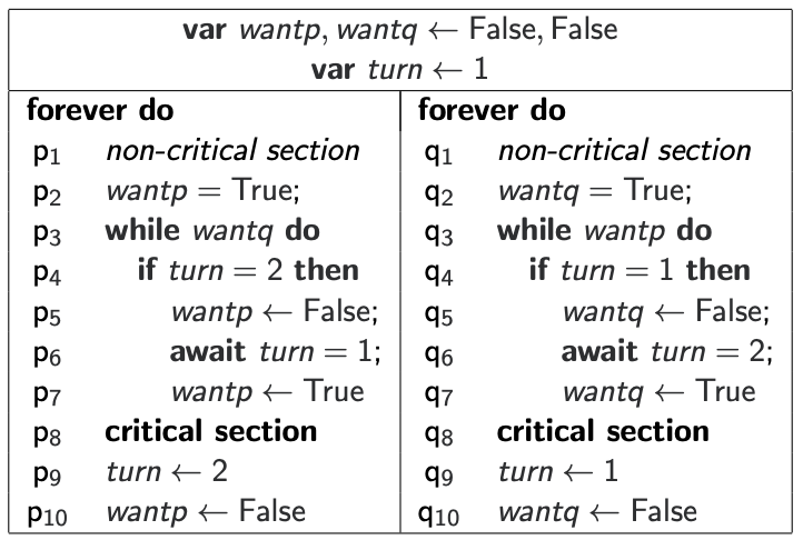
Dekker’s algorithm works well except if the scheduler pathologically tries to run the loop at q3 · · · q7 when turn = 2 over and over rather than run the process p (or vice versa).
With fairness assumption, Dekker’s algorithm is correct.
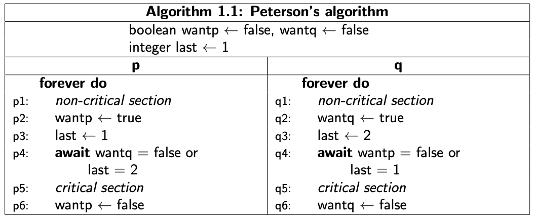
Tie-Breaker (Peterson’s) Algorithm
for 2 Processes
for n Processes
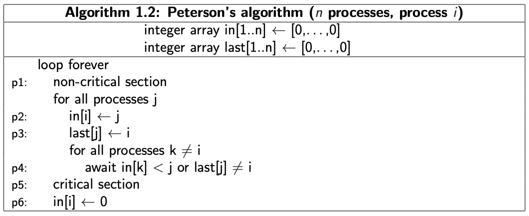
Properties of the Tie-Breaker Algorithm
Do we satisfy:
- Eventual entry? Yes
- Linear waiting? No
Linear Waiting
Linear waiting is the property that says the number of times a process is “overtaken” (bypassed) in the preprotocol is bounded by $n$ (the number of processes).
Bakery Algorithm
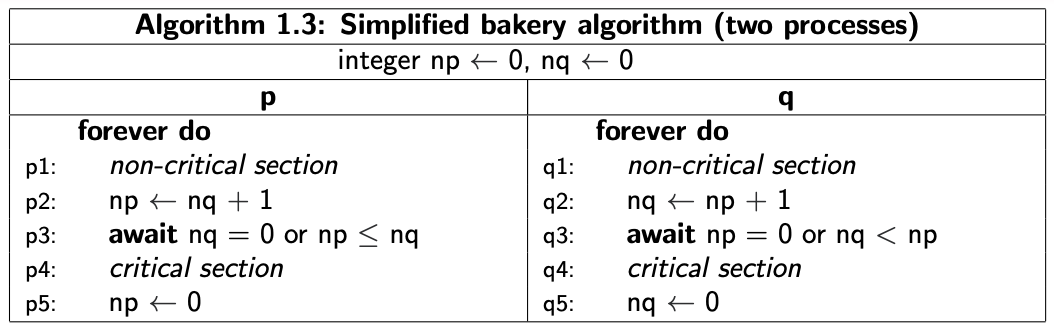
Mutual Exclusion
The following are invariants
$$
\begin{align}
np = 0&\equiv p1..2\\
nq = 0&\equiv q1..2\\
p4 &\Rightarrow nq= 0\lor np\le nq\\
q4 &\Rightarrow np= 0\lor nq\lt nq
\end{align}
$$
and hence also $¬(p4 ∧ q4)$.
Other Safety Properties
Deadlock freedom: the disjunction $nq = 0 \lor np\le nq \lor np=0\lor np\lt np$ of the conditions on the await statements at $p3/q3$ is equivalent to $T$. Hence it is not possible for both processes to be blocked there.
Absence of unnecessary delay: Even if one process prefers to stay in its non-critical section, no deadlock will occur by the first two invariants(1) and (2)
Eventual Entry
For $p$ to fail to reach its CS despite wanting to, it needs to be stuck at p3, where it will evaluate the condition infinitely often by weak fairness. To remain stuck, each of these evaluations must yield false. in LTL:
$$
\square\Diamond\neg(nq=0\lor np\le nq)
$$
Which implies
$$
(5)\space \square\Diamond nq\ne0, \text{and}\
(6)\qquad \square \Diamond nq\lt np
$$
Because there is no deadlock, (5) implies that process $q$ goes through infinitely many iterations of the main loop without getting lost in the non-critical section. But thrn it must set $nq$ to the constant $np+1$. From then onwards it is no longer possible to fail the test ($nq=0\lor np\le nq$), contradiction.
N processes
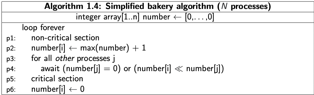
once again relying on atomicity of non-LCR lines of Ben-Ari pseudo-code; $<\!<$breaks ties using PIDs.
An Implementable Algorithm
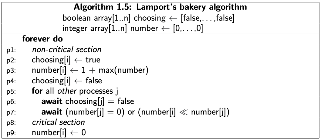
Properties of Lamport’s bakery algorithm
Cons: $O(n)$ pre-protocol; unbounded ticket numbers
Assertion 1: If $p_k 1..2 ∧ p_i5..9$ and $k$ then reaches $p_5..9$ while $i$ is still there, then number[i] < number[k].
Assertion 2: p_i8..9 ∧ p_k 5..9 ∧ i $\ne$ k ⇒ (number[i], i) $<\!<$ (number[k], k)
Fast Algorithm
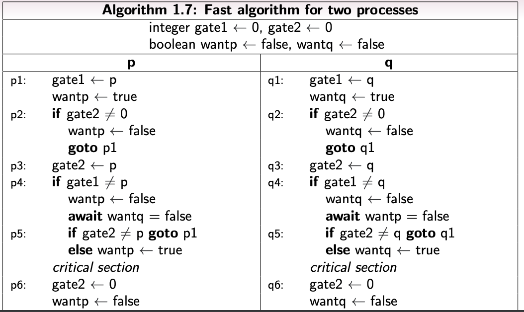
sacrifice eventual entry
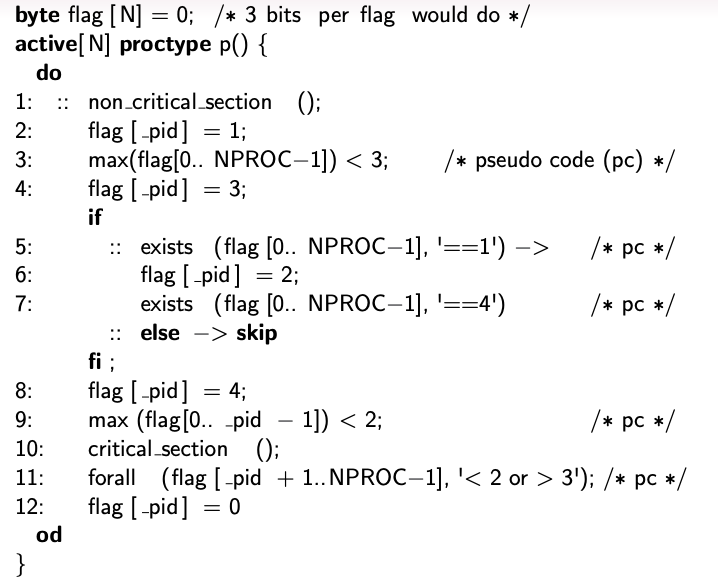
Szymanski’s Algorithm
- enforces linear wait
- requires at most $4p − \lceil{\frac{p}{n}}\rceil$ writes for p CS entries by n competing processes
- can be made immune to process failures and restarts as well as read errors occurring during writes
Phases of the pre-protocol
- announce intention to enter CS
- enter waiting room through door 1; wait there for other processes
- last to enter the waiting room closes door 1
- n the order of PIDs, leave waiting room through door 2 to enter CS
Shared variables
Each process $i$ exclusively writes a variable called flag, which is read by all the other processes. It assumes one of five values:
$0$ denoting that i is in its non-CS,
$1$ declares i’s intention to enter the CS
$2$ shows that i waits for other processes to enter the waiting room
$3$ denotes that i has just entered the waiting room
$4$ indicates that i left the waiting room
Hardware-Assisted Critical Section
Machine Instructions
Exchange
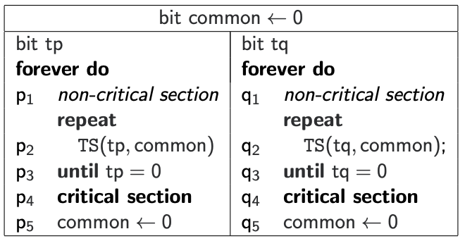
test and set
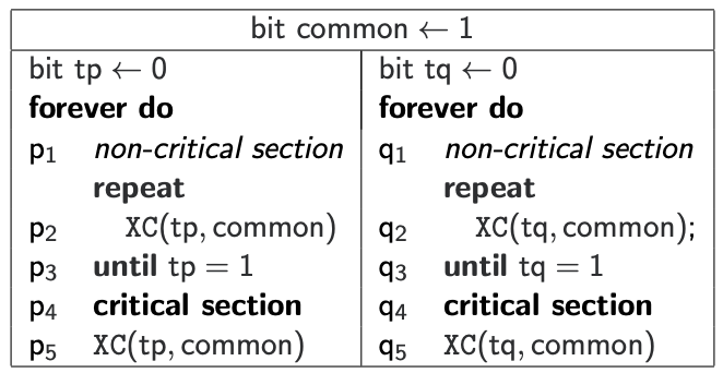
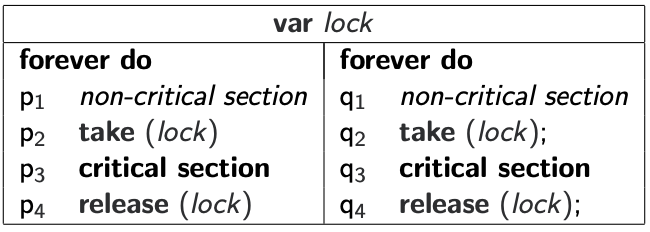
Locks
The variable common is called a lock_ (or **_mutex**). A lock is the most common means of concurrency control in a programming language implementation. Typically it is abstracted into an abstract data type, with two operations:
- Taking the lock – the first exchange (step $p_2$/ $q_2$)
- Releasing the lock – the second exchange (step $p_5$ / $q_5$)
Architectural Problems
In a mulitprocessor execution environment, reads and writes to variables initially only read from/write to cache.
Writes to shared variables must eventually trigger a write-back to main memory over the bus.
These writes cause the shared variable to be cache invalidated. Each processor must now consult main memory when reading in order to get an up-to-date value.
The problem: Bus traffic is limited by hardware.
With these instructions…
The processes spin while waiting, writing to shared variables on each spin. This quickly causes the bus to become jammed, and can delay processes from releasing the lock and violating eventual entry.