Document analysis

COMP4650 notes

Information Retrieval

“Information Retrieval (IR) is finding material (usually documents) of an unstructured nature (usually text) that satisfies an information need from within large collections (usually stored on computers).” – Manning et al.

Introduction to Boolean Retrieval

Information Retrieval

Why Information Retrieval

An essential tool to deal with information overload
Information overload

“It refers to the difficulty a person can have understanding an issue and making decisions that can be caused by the presence of too much information.” - wiki

How to perform information retrieval

Collection: A set of documents
Goal: Retrieve documents with information that is relevant to the user’s information need and helps the user complete a task

Key Objectives

Good IR system need to achieve

1. Scalability
2. Accuracy

Information Retrieval vs Natural Language Processing
| IR | NLP|
|—-|—-|
|Computational approaches|Cognitive, symbolic and computational approaches|
|Statistical (shallow) understanding of language|Semantic (deep) understanding of language|
|Handle large scale problems|(often) smaller scale problems|

IR and NLP are getting closer
IR $\Rightarrow$ NLP
– Larger data collections
– Scalable/robust NLP techniques, e.g., translation models
NLP $\Rightarrow$ IR
– Deep analysis of text documents and queries
– Information extraction for structured IR tasks

Queries and Indexing

Indexing: Storing a mapping from terms to documents
Querying: Looking up terms in the index and returning documents

Boolean query

Boolean query
E.g., “canberra” AND “healthcare” NOT “covid”
Search Procedures
Lookup query term in the dictionary

1. Retrieve the posting lists
2. Operation
   • AND: intersect the posting lists
   • OR: union the posting list
   • NOT: diff the posting list

Retrieval procedure in modern IR

1. Boolean model provides all the ranking candidates
   1. Locate documents satisfying Boolean condition
2. Rank candidates by relevance
3. Efficiency consideration
   1. Top-k retrieval

Term-document incidence matrix

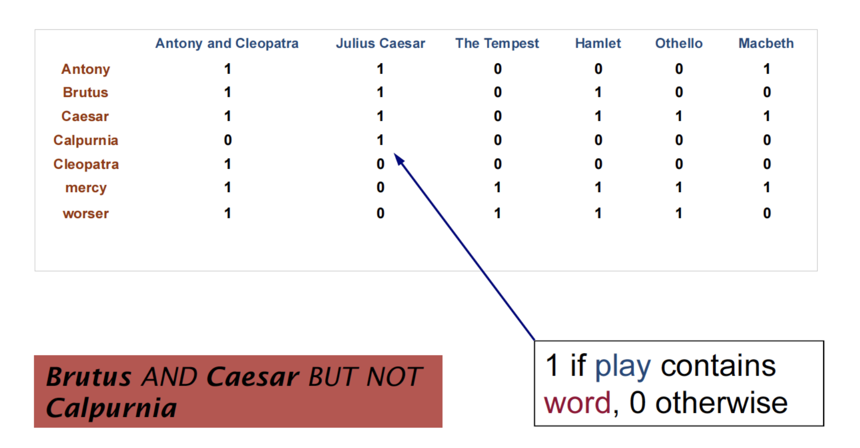
Incidence vectors

• We have a 0/1 vector for each term.
• To answer query: take the vectors for Brutus, Caesar and Calpurnia (complemented) -> bitwise AND
• 110100 AND 110111 AND 101111 = 100100

Efficiency

• Bigger Collections
  • 1 million documents
  • Each 1,000 words long
• Avg 6 bytes/word including spaces/punctuation
  • 6GB of data in the documents.
• Assume there are M = 500K distinct terms among
  these.
  • Corresponds to a matrix with 500 billion entries
  • But it has no more than one billion 1’s
  • Extremely sparse matrix!

Inverted Index

Inverted index consists of a dictionary and postings

• Dictionary: a set of unique terms
• Posting: variable-size array that keeps the list of documents given term (sorted)

INDEXER: Construct inverted index from raw text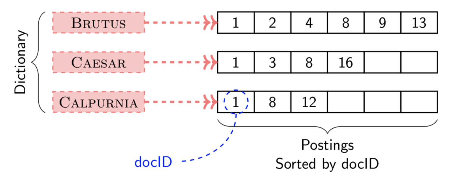

Document Tokenization

Initial Stages of Text Processing

Tokenization

Task of chopping a document into tokens

• Chopping by whitespace and throwing punctuation are not
  enough.
• Regex tokenizer: simple and efficient
• always do the same tokenization of document and query text

Normalization

Keep equivalence class of terms

• Map text and query term to same form
• U.S.A = USA = united states
• Synonym list: car = automobile
• Capitalization: ferrari $\rightarrow$ Ferrari
• Case-folding: Automobile $\rightarrow$ automobile , CAT != cat

Stemming

Stemming turns tokens into stems, which are the same regardless of inflection.

• Stems need not be realwords
• E.g. authorize, authorization; run, running

Lemmatization

Lemmatization turns words into lemmas, which are dictionary entries

Stop words removal

Stop words usually refer to the most common words in a language.

• Reduce the number of postings that a system has to store
• These words are not very useful in keyword search.

Indexer Step 1. Token sequence

1. Scan documents for indexable terms
2. Keep list of (token, docID) pairs.

Indexer Step 2. Sort tuples by terms (and then docID)
Indexer Step 3. Merge multiple term entries in a single document, Split into Dictionary and Postings, Add doc. frequency information

Boolean Retrieval with Inverted Index

Easy to retrieve all documents containing term t
Linear Intersection/union algorithm with sorted list

Boolean Retrieval

• Can answer any query which is a Boolean expression: AND, OR, NOT
• Precise: each document matches, or not
• Extended Boolean allows more complex queries
• Primary commercial search for 30+ years, and is still used

Bag-of-Words and Document Fields

we did not care about the ordering of tokens in document – Bag-of-Words (Bow) assumption
A document is a collection of words

Field (Zone) in Document

A partial solution to the weakness of BoW

• Documents may be semi-structured: Title, author, published date, body
• Users may want to limit search scope to a
  certain field

Basic Field Index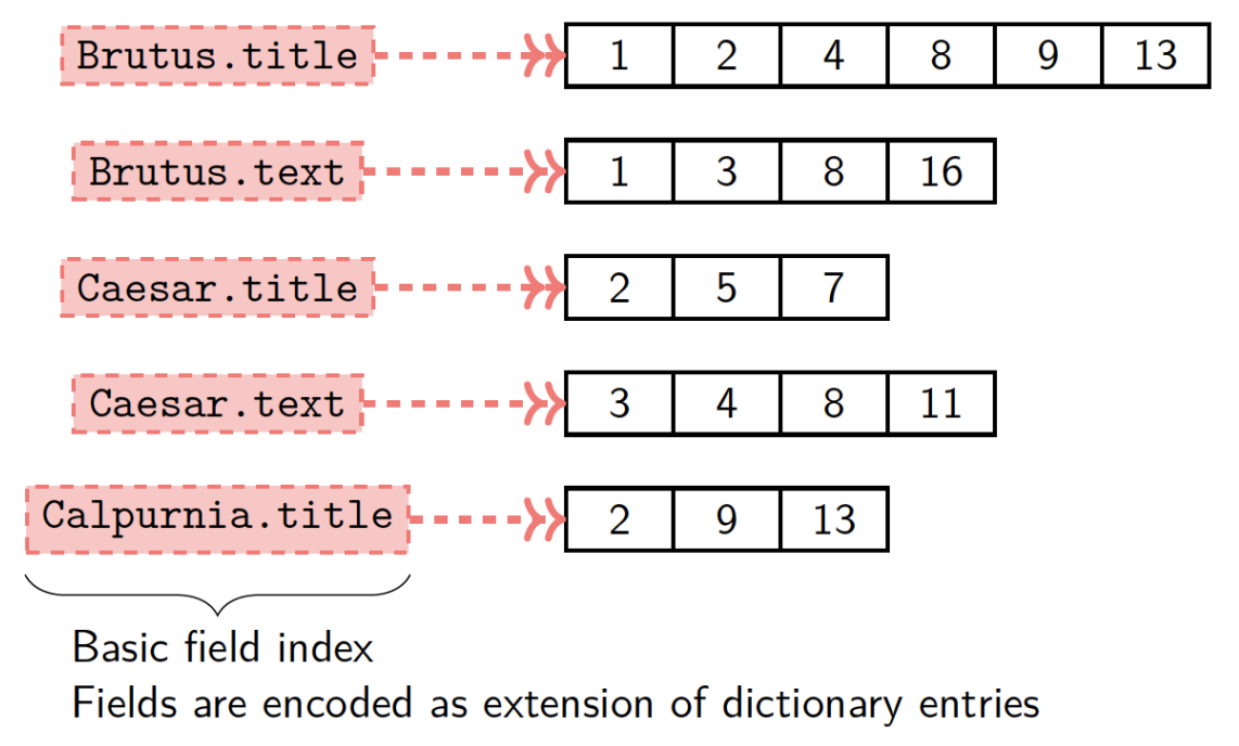

Equivalent to a separate index for each field
Field in Posting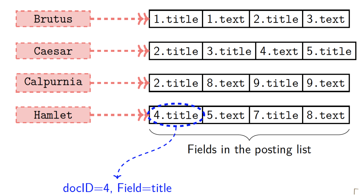

Reduces the size of the dictionary. Enables efficient weighted field scoring.

Limitations of Boolean Retrieval

• Documents either match or don’t
• Good for expert users with precise understanding of their needs and the collection
• Not good for the majority of users
  • Most users are incapable of writing Boolean queries
  • Or they find it takes too much effort
• Boolean queries often result in either too few or too many results

  Ranked Retrieval

  Given a query, rank documents so that “best” results are early in the list.
  When result are ranked a large result, we only show the top k(~10) results

Need a scoring function for document $d$ and query $q$:
$$Score(d, q)$$
Documents with a larger score will be ranked before those with a smaller score.

Weighted field scoring

term importance depends on location
Assign different weights to terms based on their location (field)!

Scoring with Weighted Fields

• $l$ fields, let $g_i$ be the weight of field $i$ and $\sum^l_{i=1}{g_i=1}$
• $t:$ a query term, $d:$ document
  $$Score(d,t)=\sum^l_{i=1}g_i\times s_i$$ ,where $s_i = 1$ if $t$ is in the field $i$ of $d$; 0 , otherwise
• A score of a query term ranges [0, 1] (because $\sum^l_{i=1}{g_i=1}$)
  In short: If a query term occurs in field $i$ of a document then add $g_i$ to the score for that document and term

Term frequency and inverse document frequency

Term Frequency

$tf_{t,d}$ is the number occurrences of term $t$ in document $d$

Rank by Term Frequency

Rank based on the frequency of query terms in documents

Let $q$ be a set of query terms ${w_1, w_2, …, w_m}$, and $d$ be a document, a term frequency score is
$$Score_{tf}(d,q)=\sum^m_{i=1}{tf_{wi,d}}$$

Importance of Terms

• Every term could have a different weight
• How can we reduce the weight of terms that occur too often in the collection

Document Frequency

Document frequency $df_t$ is the number of documents in the collection that contains term $t$

df is a good way to measure an importance of a term

• High frequency $\rightarrow$ not important (like stopwords)
• Low frequency $\rightarrow$ important
  Why not collection frequency? cf is sensitive to documents that contain a word many times

Inverse Document Frequency

Let $df_t$ be the number of documents in the collection that contain a term $t$. The inverse document frequency (IDF) can be defined as follows:
$$idf_t=log\frac{N}{df_t}$$,
where $N$ is the total number of documents

The idf of a rare term is high, whereas the idf of a frequent term is likely to be low

TF-IDF & WF-IDF

The tf-idf weight of term $t$ in document $d$ is as follows:
$$tf-idf_{t,d}=tf_{t,d}\times idf_t$$

Using tf-idf weights, the score of document $d$ given query $q = (t_1, t_2, …, t_m)$ is:
$$Score_{tf-idf}(d,q)=\sum^m_{i=1}tf-idf_{ti,d}$$

Sublinear tf scaling
Use logarithmically weighted term frequency (wf)
$$wf_{t,d}= tf_{t,d} > 0? 1+log(tf_{t,d}): 0$$
Logarithmic term frequency version of tf-idf
$$wf-idf_{t,d}=wf_{t,d}\times idf_f$$

Limitation

1. tf-idf relies heavily on term frequency
2. tf-idf score increases linearly with term frequency
   Claim: the marginal gain of term frequency should decrease as term frequency increases.

• The relationship should be non-linear

3. Bothe tf-idf and wf-idf prefer longer documents

Maximum tf normalization
Let $tf_{max}(d)$ be the maximum frequency of any term in document $d$
Normalized term frequency is defined as
$$ntf_{t,d}=\alpha+(1-\alpha)\frac{tf_{t,d}}{tf_{max}(d)}$$
The value of ntf is in [1, $\alpha$]
Note: it can be skewed by a single term that occurs frequently

Vector space IR model

Document as Vectors
Given a term-document matrix, a document can be represented as a vector of length $V$, where $V$ is the size of vocabulary
Document Similarity in Vector Space

• Distance from vector to vector
• Angle difference between vectors
  • Cosine similarity:
    $$sim(\overrightarrow d_1, \overrightarrow d_2)=\frac{\overrightarrow d_1 \bullet \overrightarrow d_2}{|\overrightarrow d_1|\times|\overrightarrow d_2|}$$
    Standard way of quantifying similarity between documents, 1 if directions of two vectors are the same, 0 if directions of two vectors are orthogonal
    Cosine similarity is not sensitive to vector magnitude

Why not euclidean distance
Euclidean distance is sensitive to the vector magnitude
The Euclidean distance of normalized vectors is proportional to cosine similarity.
Query as a vector

• Pretend it is a document
• When using tf-idf the document frequency for the query vector comes from the document collection
• We can compute the similarity between the query vector and document vector using cosine similarity

Score Function of Vector Space Model
$$Score_{vsm}(d,q)=sim(\overrightarrow{d},\overrightarrow{q})$$
We use the cosine similarity with the query to rank documents.

Evaluation of IR systems

Purpose of evaluation

To build IR systems that satisfy user’s information needs
Given multiple candidate systems, decide the best one
What do we want to evaluate

• System Efficiency
  • Speed
  • Storage
  • Memory
  • Cost
• System Effectiveness
  • Quality of search result
  • relevance
  • hit rates

Test collection

A test collection is a collection of relevance judgment on (query, document) pairs. This relevancy information is known as the ground truth. It is typically constructed by trained human annotators.

Three Components of Test Collections

• A collection of documents
• A test suite of information needs, expressible as queries
• A set of relevance judgment; a binary assessment of either relevant or irrelevant for each query-document pair

Relevance Judgment

• Relevance is assessed relative to an information need, not a query
• A document is relevant if it addresses the
  information need.
• The document does not need to contain
  all/any of the query terms

Two evaluation settings:

• Evaluation of unranked retrieval sets (Boolean retrieval)
  • Ranks of retrived documents are not important
  • Retrieved (returned) documents vs. Not retrieved documents
• Evaluation of ranked retrieval sets
  • Rank of retrieved documents are important
  • Relevant documents should be ranked above irrelevent documents

    Evaluation of unranked retrieval sets

Contingency Table

a summary table of retrieval result

	Relevant	Not relevant
Retrieved	true postive(tp)	false postive(fp)
Not retrieved	false negative(fn)	true nagative(tn)

• tp: Number of relevant documents returned by system
• fp: Number of irrelevant documents returned by system
• fn: Number of relevant documents not returned by system
• tn: Number of irrelevant documents not returned by system

Precision, Recall, and Accuracy

Precision: fraction of retrieved documents that are relevant

$$Precision=\frac{tp}{tp+fp}$$

Recall: fraction of relevant documents that are retrieved

$$Precision=\frac{tp}{tp+fn}$$

Accuracy: fraction of relevant documents that are correct

$$Accuracy=\frac{tp+tn}{tp+tn+fp+fn}$$
Accuracy is not appropriate for IR because we don’t care irrelevant results
F-Measure

a single measure that trades off precision and recall
$$F=\frac{1}{\alpha\frac{1}{p}+(1-\alpha)\frac{1}{R}}, \alpha\in[0,1]$$

This is the weighted harmonic mean of precision(P) and recall(R)

• $α > 0.5$: emphasises precision, e.g., $(α = 1)$ Precision
• $α < 0.5$: emphasises recall, e.g., $(α = 0)$ Recall

F1-measure: the harmonic mean of precision and recall $(α = 0.5)$
$$F=\frac{2PR}{P+R}$$

Evaluation of ranked retrieval sets

Precision-Recall Curve
Compute recall and precision at each rank k (i.e. using the top k docs)
Plot (recall, precision) points until recall is 1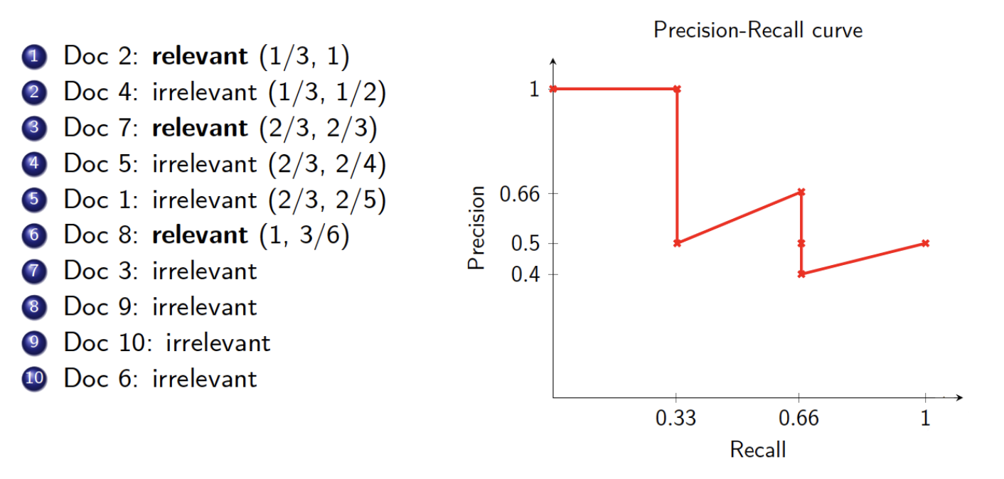

Interpolated Precision-Recall
At a given recall level use the maximum precision at all higher recall levels.
Makes it easier to interpret
Intuition: There is no disadvantage to retrieving more documents if both precision and recall improve.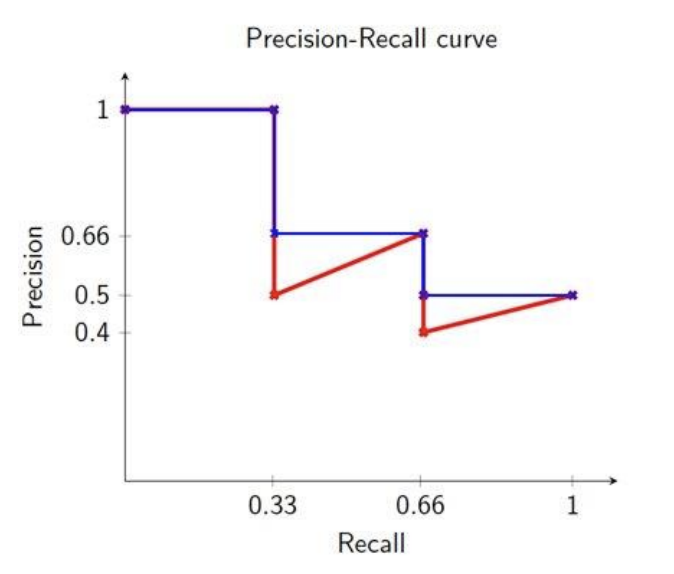

For system evaluation we need to average across many queries. It is not easy to average a PR curve in its current form.
Solution:
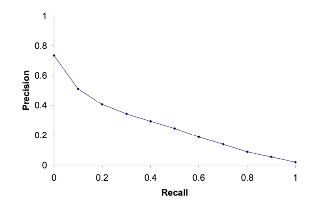
11-point interpolated PR curve. Interpolated precision at 11 different recall points.
For system evaluation:

• Each point in the 11-point interpolated precision is averaged across all queries in the test collection
• A perfect system will have a straight line from (0,1) to (1,1)
  

Single Number Metrics
Average Precision

Average Precision is the area under the uninterpolated PR curve for a single query.

MAP

Mean Average Precision (MAP) is the mean of the average precision for many queries.

• MAP is a single figure metric across all recall levels.
• Good if we care about all recall levels

Mean Reciprocal Rank (MRR)

Averaged inverse rank of the first relevent document.
For if we only care about how high in the ranking the first relevant document is.

Other ranking measures

• Precision at K
  • Average precision at top k documents
• Recall at K
  • Average recall at top k documents
• Receiver Operating Characteristics (ROC) curve
• Normalized Discounted Cumulative Gain (NDCG)
  • Requires graded relevance judgement

Web basics

The Web and Other Networks

Documents on the web are linked by hyperlinks.
Academic papers are linked by citations and co-authorship relations.
Legal documents are linked by citations.
Online users are linked by interactions or formal social network ties.

Nodes and Edges

Nodes represent entities (e.g. documents, people)
Edges are relationships between nodes. (e.g. hyperlinks, co-authorship relations)
Edges can be directed (go in a specific direction)

Degree of a Node

• Degree: the number of edges connected to a node
• In-degree: the number of edges going to a node
• Out-degree: the number of edges coming from a node.

Link Analysis

• Link analysis uses information about the structure of the web graph to aid search
• It is one of the major innovations in web search.
• It was one of the primary reasons for Google’s initial success.

  Citation Analysis

• Many documents include bibliographies with citations to other previously published documents
• Using citations as edges, a collection of documents can be viewed as a graph.
• The structure of this graph can provide interesting information about the similarity of documents and the structure of information. Even when document content is ignored

Impact Factor of a Scientific Journal

measure the importance (quality, influence) of scientific journals
A measure of how often papers in a journal are cited
Computed and published annually by the

Institute for Scientific Information
The impact factor of a journal $J$ in year $Y$ is the average number of citations (from indexed documents published in year $Y$) to a paper published in $J$ in year Y−1 or Y−2.
Does not account for the quality of the citing article.

Bibliographic Coupling

Measure of similarity of documents introduced by Kessler in 1963.
The bibliographic coupling of two documents A and B is the number of documents cited by both A and B.
Size of the intersection of their bibliographies.

Co-Citation

An alternate citation-based measure of similarity introduced by Small in 1973
Number of documents that cite both A and B.

Citations vs. Link

• Many links are navigational
• Many pages with high in-degree are portals not content providers
• Not all links are endorsements
• Company websites don’t point to their competitors
• Citations to relevant literature is enforced by peer-review.

  Authorities and Hubs: HITS algorithm

Authorities

Authorities are pages that are recognized as providing significant, trustworthy, and useful information on a topic.

In-degree (number of pointers to a page) is one simple measure of authority

• However, in-degree treats all links as equal.

Hubs

Hubs are index pages that provide lots of useful links to relevant content pages (authorities).

HITS

Determines hubs and authorities for a particular topic through analysis of a relevant subgraph

Based on mutually recursive, assumptions:

• Hubs point to lots of authorities.
• Authorities are pointed to by lots of hubs

HITS Algorithm

Computes hub and authority scores for documents on a particular topic

• The topic is specified by a query
• Relevant pages from the query are used to construct a base subgraph S.
• Analyze the link structure of pages in S to find authority and hub pages.

Constructing a Base Subgraph S:

1. For a specific query, let the set of documents returned by a standard search engine be called the root set R.
2. Initialize S to R.
3. Add to S all pages pointed to by any page in R
4. Add to S all pages that point to any page in R.

Base Limitations:

• To limit computational expense:
  • Limit the number of root pages to the top 200 pages retrieved for the query
  • – Limit the number of “back-pointer” pages to a random set of at most 50 pages returned by a “reverse link”
• To eliminate purely navigational links
  • Eliminate links between two pages on the same host.
• To eliminate “non-authority-conveying” links:
  • Allow only m ($m \in[4,8]$) pages from a given host as pointers to any individual page query

Authorities and In-Degree
Even within the base set S for a given query, the nodes with highest in-degree are not necessarily authorities (may just be generally popular pages like Yahoo or Amazon)
Authority pages are pointed to by several hubs (i.e. pages that point to lots of authorities).

Iterative Algorithm
Use an iterative algorithm to slowly converge on a mutually reinforcing set of hubs and authorities:

• Maintain for each page $p\in S$:
  • Authority score: $a_p$ (vector a)
  • Hub score: $h_p$ (vector h)
• Initialize all $a_p=h_p=1$
• Maintain normalized scores:
  $\sum_{p\in S}(a_p)^2=1$
  $\sum_{p\in S}(h_p)^2=1$

HITS Update Rules

• Authorities are pointed to by lots of good hubs
  • $a_p=\sum_{q:q\rightarrow p}h_q$
• Hubs point to lots of good authorities:
  • $h_p=\sum_{q:p\rightarrow q}a_q$

HITS Iterative Algorithm
Initialize for all $p \in S: a_p = h_p = 1$
For $i = 1$ to $k$:

• For all $p \in S$: $a_p=\sum_{q:q\rightarrow p}h_q$ (update auth. scores)
• For all $p\in S$: $h_p=\sum_{q:p\rightarrow q}a_q$(update hub scores)
• For all $p\in S$: $a_p= a_p/c, c: \sum_{p\in S}(a_p/c)^2=1$ (normalize a)
  For all $p\in S$: $h_p= h_p/c, c: \sum_{p\in S}(h_p/c)^2=1$ (normalize h)

Convergence

• Algorithm converges to a fix-point if iterated indefinitely.
• Define A to be the adjacency matrix for the subgraph defined by S.
  • $A_{ij} = 1$ for $i \in S, j \in S$ iff $i\rightarrow j$
• Authority vector, $a$, converges to the principal eigenvector of $A^TA$
• Hub vector, $h$, converges to the principal eigenvector of $AA^T$
• In practice, 20 iterations produces fairly stable results

Finding Similar Pages Using Link Structure

• Given a page, P, let R (the root set) be t (e.g. 200) pages that point to P.
• Grow a base set S from R.
• Run HITS on S.
• Return the best authorities in S as the best similar-pages for P
• Finds authorities in the “link neighborhood” of P

PageRank

Does not attempt to capture the distinction between hubs and authorities
Gives each page a score which measures authority
Applied to the entire document corpus rather than a local neighborhood of pages surrounding the results of a query

PageRank Algorithm
Let $S$ be the total set of pages.
Let $\forall p\in S:E(p)=\alpha/|S|$ (for some $0<\alpha<1$)
Initialize $\forall p\in S: R(p) = 1/|S|$
Until ranks do not change (much) (convergence)
For each $p\in S$:
$R’(P)=[(1-\alpha)\sum_{q:q\rightarrow p}\frac{R(q)}{N_q}+E(p)$
$c=1/\sum_{p\in S}R’(p)$
for each $p\in S: R(p) = cR´(p)$ (normalize)

• $N_q$ is the total number of out-links from page q.
• A page, q, “gives” an equal fraction of its authority to all the pages it points to (e.g. p).
• c is a normalizing constant set so that the rank of all pages always sums to 1
• a “rank source” E that continually replenishes the rank of each page, p, by a fixed amount E(p)

Speed of Convergence
Number of iterations required for convergence is empirically O(log n) (where n is the number of links). Therefore, calculation is efficient

Machine Learning

ML Intro and notation

Supervised Learning

Goal: given both the inputs and the outputs for a training dataset, find a function h of the inputs that that returns the correct output (or as close as possible)

Categorical output $\Rightarrow$ classification problem

Scalar output $\Rightarrow$ regression problem

Terminology

dataset, corpus, training set, collection, set of examples

Objects (samples, observations, individuals, examples, data points)

Variables (attributes, features) = describes a objects

Dimension = number of variables

Size = number of objects

Notation

examples / data points / input	$𝒙^{(1)} ,…, 𝒙^{(𝑛)}$ ~$X$
labels / annotations / target	$y^{(1)} ,…, y^{(𝑛)}$~$Y$
predicator / model	𝑓$_w$ 𝒙 : 𝑋 $\rightarrow$ Y
features of datapoint k	𝒙$^{(𝑘)}$ = (𝑥$_1^{(𝑘)}$ ,𝑥$_2^{(𝑘)}$ …. ,𝑥$_m^{(𝑘)}$ )
Predictions from the model	$\hat y$ = 𝑓$_w($𝒙$)$

Bold denotes vectors

Linear Regression

We find the best linear function to model our data points

To make a prediction for a new point we just evaluate our function at that point

What do we need?

1. A way of expressing linear functions

2. A way to measure how well the line fits the data (called a loss function)

3. A way to find the line with the smallest loss given the data

   Gradient descent

Linear Functions:

One Feature

A straight line can be written $\hat y=wx+b$

• 𝑤 - is the slope of the line (parameter)
• 𝑥 - is the feature (input)
• 𝑏 - is the bias (parameter)
• $\hat y$ - is the prediction of the target variable (output)

Many Features

We can have a linear function with many features:

$\hat y=𝑤_1𝑥_1 + 𝑤_2𝑥_2 + 𝑤_3𝑥_3+… +b$

Written more compactly for 𝑚 features:

$\hat y = b+\sum_{i=0}^m w_ix_i$

Written in vector form with vectors $\vec w$ and $\vec x$:

$\hat y = b+\vec w\vec x$

Multiple Linear Regression

If we have more than one target per example, then we can use a different set of parameters for each target:

$$\hat y_1=𝑤_{1,1}𝑥1 + 𝑤{1,2}𝑥2 + 𝑤{1,3}𝑥_3+… +b$$

$$\hat y_2=𝑤_{2,1}𝑥1 + 𝑤{2,2}𝑥2 + 𝑤{2,3}𝑥_3+… +b$$

$$\hat y_3 = w_{3,1}𝑥1 + w{3,2}𝑥2 + w{3,3}𝑥_3+… +b$$

In matrix/vector form this is (for matrix $W$, and vectors: $\vec {\hat y}$ , $\vec x$, $\vec b$):

$\hat y = b+W\vec x$

Loss Function

Measures how well the line models the data:

$𝐿 = \sum_{i=1}^𝑛 (\hat y^{(𝑖)} − 𝑦^{(𝑖)})^2$

$𝐿 = \sum_{i=1}^𝑛 (wx^{(𝑖)}+b − 𝑦^{(𝑖)})^2$

$𝒙^{(𝑖)}$ - the features of the i’th datapoint

$𝑦^{(𝑖)}$ - the ground truth target of the i’th datapoint

$\hat y^{(𝑖)}$ - the predicted target of the i’th datapoint

Optimization

We have a loss function 𝐿 which measures how good a particular line (𝑤, 𝑏) is for our training dataset D

We want to solve: argmin$_{𝑤,𝑏}$ 𝐿(𝑤, 𝑏,𝐷)

There are many different algorithms for solving optimization problems, gradient descent is a very popular one when everything is differentiable

Gradient Descent

A greedy strategy for optimization

Start by picking values for 𝑤 and 𝑏, e.g. by sampling from𝑁(0,1).

Then compute the gradients $\frac{𝑑𝐿}{𝑑𝑤}$ and $\frac{𝑑𝐿}{𝑑𝑏}$

Then update:

$w:=w-\alpha \frac{𝑑𝐿}{𝑑𝑤}$

$b:=b-\alpha \frac{𝑑𝐿}{𝑑b}$

𝛼 is the learning rate, it controls how much the values change each step.

The role of learning rate

The learning rate 𝛼 is a hyper-parameter that you set, it controls how much the weights are changed in each step.

Too small 𝛼 ⇒ need to take many steps.

Too large 𝛼 ⇒ may not converge.

Multinomial Logistic Regression

Classification

To use a linear model 𝑊𝒙 + 𝒃 (multiple linear regression)

We can modify the task to predicting the probability that an example belongs to each class.

Suppose that each point can be labelled with one of 𝑂 different classes. Then our model $\bar P$(𝒚|𝒙) = 𝑊𝒙 + 𝒃 outputs a vector of size $O$.

$\bar P$ denotes unnormalized probabilities. (often called logits). These may be negative.

From Logits to Probabilities

The output values of the linear model are not probabilities:

• Need all the output values to be non-negative.
• Need output values to sum up to 1.

$$softmax(v)i=\frac{exp(v_i)}{\sum^o{j=0}exp(v_j)}$$

Step 1: Apply exp to all values. This makes them positive

Step 2: Divide each value by the sum of all values. This makes them sum to 1.

The result is a categorical probability distribution

Multinomial Logistic Regression

$P(y \mid x)$ = softmax (𝑊𝒙 + 𝒃)

Classification: Loss

Compute loss between our predicted probabilities and onehot encoding of class label $y$, i.e. the probability of the correct class should be 1, all others should be 0.

$L$(softmax 𝑊𝒙 + 𝒃 , 𝒚)

Classification: Cross-Entropy

We could use the sum of squared differences as our loss function, just like for regression.

In practice, using cross-entropy as the loss function for classification gives better results.

Cross entropy for one datapoint:

CrossEntropy(𝒙, 𝒚)=$-\sum_{i=1}^oy_ilogP(y_i\mid 𝒙)$

Classification: Prediction

To make a prediction for a new data point

using the model compute probabilities for each class.

predict the class with the largest probability.

Representation in NLP

Representation

Text represented as a string of bits/characters/words is hard to work with

• Variable length
• High dimensional
• Similar representations may have very different meanings

Meaning

Meaning in language is:

• Relational (based on relationships)
• Compositional (built from smaller components)
• Distributional (related to usage context)

Simple document representation

Document Representation

• We can represent documents as vectors of the words/terms they contain (BoW model)
  • Vector may be
    • Binary occurrence
    • Word count
    • TFIDF scores
  • The vector representation may be the size of the vocabulary ~ 50000 words is common
  • Very inefficient for many documents
  • Fortunately, most documents do not contain most words so we can use a sparse representation with tuples of the form: (term_id, term_count) for tuples where term_count > 0

Word representation

Word Representation (One-hot)

• In traditional NLP, we regard words as discrete symbols

• Vector dimension = number of words in vocabulary

  hotel = 10 = [0 0 0 0 0 0 0 0 0 0 1 0 0 0 0]

  motel = 7 = [0 0 0 0 0 0 0 1 0 0 0 0 0 0 0]

• issue: Similar words do not have similar vectors

Context-based Word Representation

• Sentence
• Window
  • Use k words on either side of the focal word as the context
• Word Co-occurrence Matrix
  • A co-occurance matrix of words gives a vector representation for each word.
  • This gives equal importance to all context words
  • Weighting
    • tf-idf
    • PPMI: Positive Pointwise Mutual Information (more common)

Pointwise Mutual Information

The ratio of the probability that the words occur together compared to the probability that they would occur together by chance

The amount of information the occurrence of a word $𝑤_𝑖$ gives us about the occurrence of another word $𝑤_𝑗$ . (and vise versa)

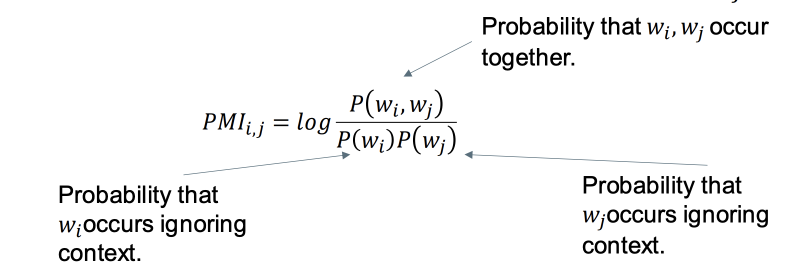
PMI can be negative when words occur together less frequently than by chance.

Typically, negative values are not reliable. We set them to 0:

𝑃𝑃𝑀𝐼 = max(0,𝑃𝑀𝐼)

Similarity with Pointwise Mutual Information

𝑠𝑖𝑚(x, y) = cos($𝑣_x,𝑣_y$)

Drawbacks of a Sparse Representation

• The raw count / tf-idf / PPMI matrix is:

  High dimensional, thus more difficult to use in practice.

• Suffers from sparsity. Hard to find similarity between words

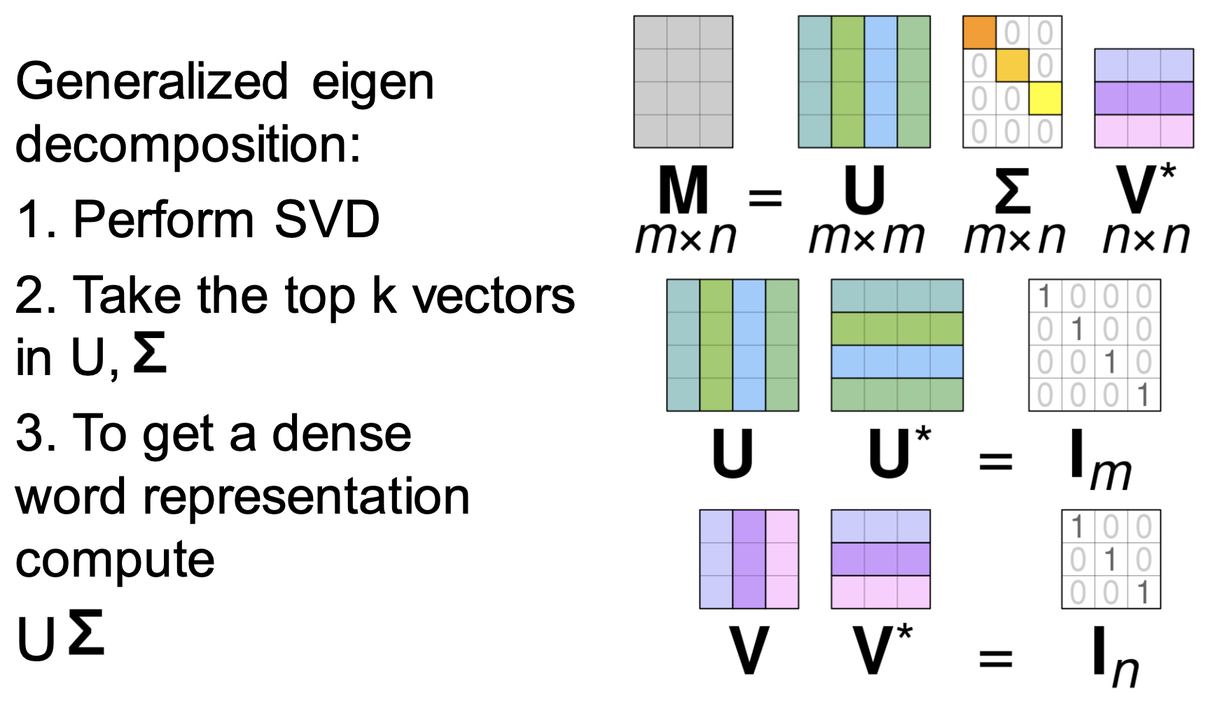
Singular Value Decomposition

reduce the dimensionality of a word-word co-occurrence matrix

Word2Vec

Word Representation (Word Vector)

dense word vectors are sometimes called word embeddings or word representations. They are distributed representations. Typical number of dimensions: 64, 128, 256, 300, 512, 1024

Several Word2Vec Algorithms: Most common is skip-gram with negative sampling

Approach:

• A self-supervised classification problem
• We learn word embeddings to do classification
• In the end we care only about the embeddings

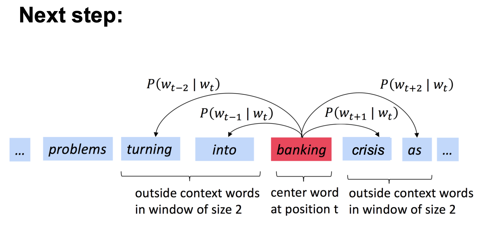
Skip-gram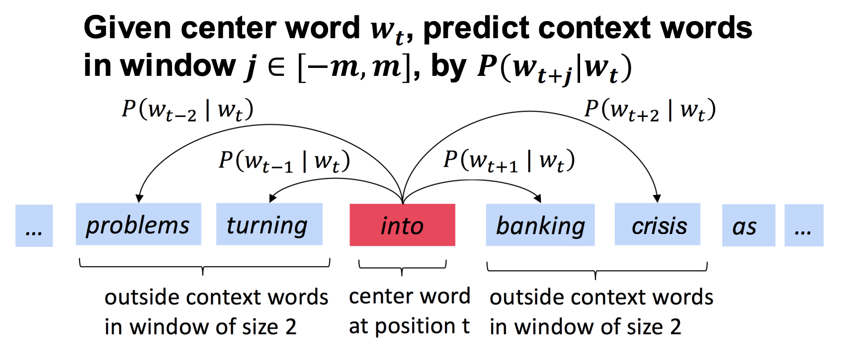

Word2Vec as Logistic Regression

Word2Vec uses a multinomial logistic regression classifier (without a bias term):

P(y | x) = softmax($𝑊x$)

Here $y$ is the context word and $x$ is an embedding of the center word.

In this model we can interpret the matrix $W$ as being composed of embedding of the context words

Model

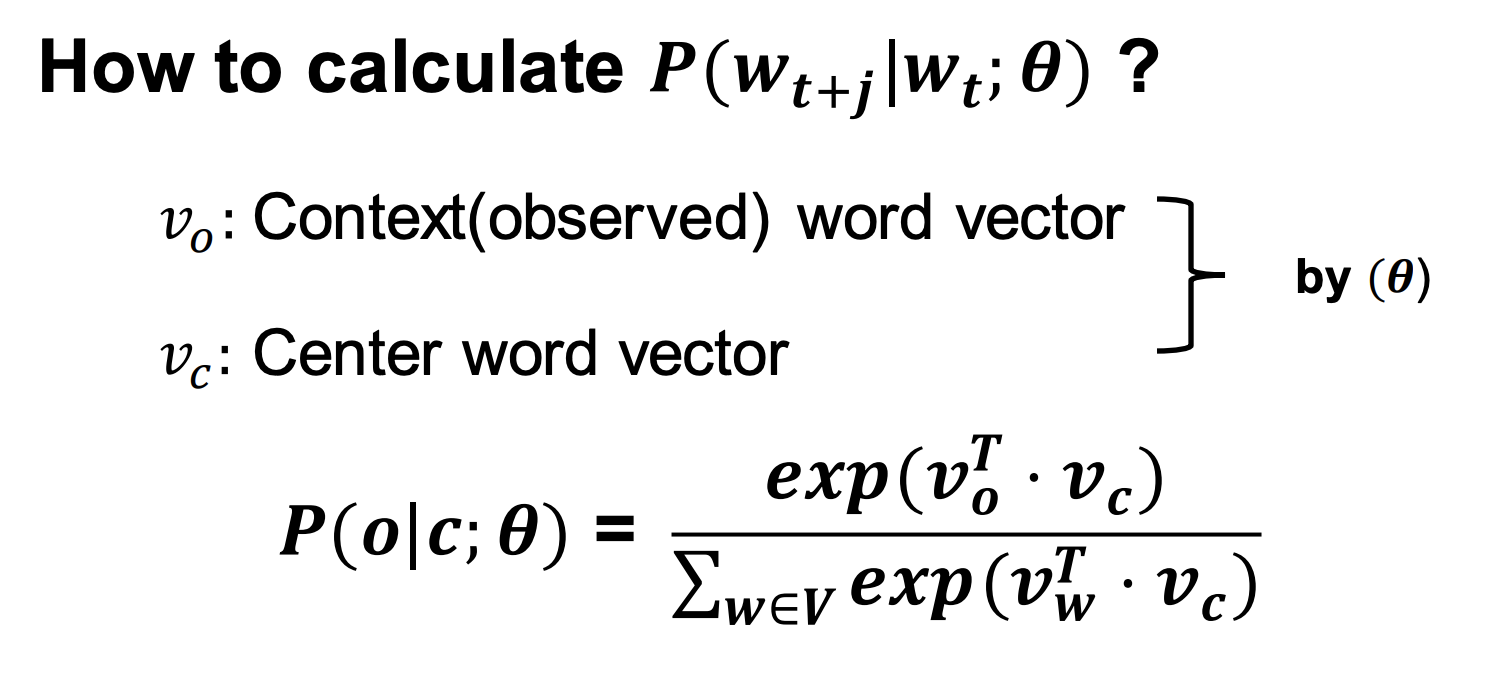
Once trained with cross-entropy loss we use $𝑣_𝑐$ as the word embedding and throw everything else away.

Word2Vec

When we train word2vec we also train the center word embeddings

How:

• Start with random embeddings
• Backpropagation to compute gradient (next lecture)
• Gradient descent

Loss function (average cross entropy):

Natural Language Processing

Language Modelling

• Goal: assign a probability to a word sequence
  • Speech recognition
  • Spelling correction
  • Collocation error correction
  • Machine Translation
  • Question-answering, summarisation, image capturing etc

Probabilitistic Language Modelling

A language model computes the probability of a sequence of words

• A vocabulary $V$
• $p(x_1, x_2, \dots, x_l)\ge 0$
• $\sum p(x_1, x_2, \dots, x_l)=1$

Related task: probability of an upcoming word ($p(x_1\mid x_1, x_2, x_3)$)

LM: Either $p(x_1\mid x_1, x_2, x_3)$ or $p(x_1, x_2,\dots, x_l)$

Probability Calculation

Chain rule

To compute $p(x_1, x_2, …, x_l)$ use Chain rule:
$$
p(x_1, x_2, …, x_l)=p(x_1)p(x_2|x_1)p(x_3|x_1,x_2)\dots(x_l|x_1,…,x_{l-1})
$$
Drawbacks: it is likely that the whole context $(x_1, x_2, …, x_l)$ doesn’t appear in the data, resulting the probability of $0$.

Markov Assumption

simplifying assumption

instead of using the whole context, use one or two most recent words

Zero-order Markov assumption(Unigram Model)
$$
P(x_1, x_2, \dots, x_l)=P(x_1)\underset{i=1}{\overset{l}\Pi}P(x_i)
$$

• Not very good

First-order Markov assumption (Bigram Model):

Assumes only most recent words are relevant

$$
\begin{align}
P(x_1, x_2, \dots, x_l)&=P(x_1)\underset{i=2}{\overset{l}\Pi}P(x_i\mid x_1,…,x_{x-1})\
&=P(x_1)\underset{i=2}{\overset{l}\Pi}P(x_i\mid x_{x-1})
\end{align}
$$

• Maximum likelihood estimation:
  $$
  P(x_i\mid x_{i-1})=\frac{count(x_{i-1}, x_i)}{count(x_i)}
  $$

• Log probabilities:

  • logP(I want to eat) = logP(I)+logP(want|I)+logP(to|want)+logP(eat|to)
  • using log can make probabilities in a certain range (it won’t be very small)
  • Log helps with numerical stability (probabilities get small)

Second-order Markov assumption (Trigram Model):
$$
P(x_1, x_2, \dots, x_l)=P(x_1)\underset{i=1}{\overset{l}\Pi}P(x_i|x_{i-1},x_{i-2})
$$

• can handle long-distance of language
• can extend to 4-gram, 5-gram…

Sequence Generation

Compute conditional probabilities:

e.g. P(want|I) = 0.32

Sampling:

• Ensures you don’t just get the same sentence all the time
• Generate a random number in [0,1] (based on a uniform distribution)
• Words are better fit are more likely to be selected

Interpolation

mix lower order n-gram probabilities

$\lambda$s are hyperparameters

To handle the unseen words and the issue of $0$ probability (phrase with $0$ probability but single word may not)

Bigram models:
$$
\hat P(x_i\mid x_{x-1})=\lambda_1P(x_i\mid x_{i-1})+\lambda_2P(x_i\mid x_{i})\
\lambda_1\ge 0, \lambda_2\ge 0\
\lambda_1+\lambda_2=1
$$
Trigram models:
$$
\hat P(x_i\mid x_{x-1}, x_{i-2})=\lambda_1P(x_i\mid x_{i-1}, x_{i-2})+\lambda_2P(x_i\mid x_{i-1})+\lambda_3P(x_i\mid x_{i})\
\lambda_1\ge 0, \lambda_2\ge 0, \lambda_2\ge 0\
\lambda_1+\lambda_2+ \lambda_30=1
$$
How to fit $\lambda$s

• Estimate $\lambda_i$ on held-out data

  Training data, held-out data, test data

• Typically use Expectation Maximization (EM)

• One crude approach
  $$
  \begin{align}
  \lambda_1&=\frac{count(x_{i-1}, x_{i-2})}{count(x_{i-1}, x_{i-2})+\gamma}\
  \lambda_2&=(1-\lambda_1)\times\frac{count(x_{i-1})}{count(x_{i-1})+\gamma}\
  \lambda_3&=1-\lambda_1-\lambda_2\
  \end{align}
  $$

  • Ensures $\lambda_i$ is larger when count is larger
  • Different lambda for each n-gram
  • Only one parameter to estimate ($\gamma$)

Absolute-Discounting Interpolation

We tend to systematically overestimate n-gram counts

$\longrightarrow$ we can use this to get better estimates and set lambdas. Using discounting

• Involves the interpolation of lower and higher-order models

• Aims to deal with sequences that occur infrequently

• Subtract $d$ (the discount, typically $0.75$) from each of the counts
  $$
  P_{AbsDiscount}(x_i\mid x_{x-1})=\frac{count(x_{i-1}, x_i)-d}{count(x_i)}+\lambda(x_{i-1})P(x_{i-1})
  $$

• The discount reserves some probabilities mass for the lower order n-grams

  • Thus, the discount determines the $\lambda$

Kneser-Ney Smoothing

• A techique built on top of Absolute-Discounting Interpolation.

• “Smoothing” $\rightarrow$ Adjust low probs upwards and high probs downwards

• If there are only a few words that come after a context, then a novel word in that context should be less likely

• But we also expect that if a word appears after a small number of contexts, then it should be less likely to appear in a novel context

Works well and also used to improve NN approaches.

• Provides better estimates for probabilities of lower-order unigrams:

$P_{continuation}(X)$

How likely is a word to continue a new context?

• For each word $x_i$, count the number of bigram types it completes
  $$
  P_{continuation}(x_i)\propto\mid{x_{i-1}\mid count(x_{i-1}, x_i)}\mid
  $$
  i.e. the unigram probability is proportional to the number of different words it follows

• Normalized by the total number of bigram types:
  $$
  \mid{(x_{j-1}, x_j)\mid count(x_{i-1}, x_i)>0}\mid\
  P_{continuation}(x_i)=\frac{\mid{x_{i-1}\mid count(x_{i-1}, x_i)}\mid}{\mid{(x_{j-1}, x_j)\mid count(x_{i-1}, x_i)>0}\mid}
  $$
  Estimate of how likely a unigram is to continue a new context

Kneser-Ney Smoothing

definition for bigrams:
$$
P_{KN}(x_i\mid x_{i-1})=\frac{max(count(x_{i-i},x_i)-d, 0)}{count(x_{i-1})}+\lambda(x_{i-1})P_{continuation}(x_i)
$$
where
$$
\lambda(x_{i-1})=\frac{d}{count(x_{i-1})}\mid{x\mid count(x_{i-1},x)>0}\mid
$$
Stupid Backoff

Smoothing for web-scale N-grams

• No discounting, just use relative frequencies!

• Does not give a probability distribution (Gives a score)
  $$
  S(w_i\mid w^i_{i-k+1})=
  \begin{cases}
  \frac{count(w^i_{i-k+1})}{count(w^{i-1}{i-k+1})} \text{ if }count(w^i{i-k+1})>0\
  0.4S(w_i\mid w^i_{i-k+2})\text{ otherwise}
  \end{cases}\
  S(w_i)=\frac{count(w^i)}{N}
  $$
  $N$ is the size of the training corpus in words